MTH252
Data Structures and Algorithms II

MTH252
Data Structures and Algorithms II
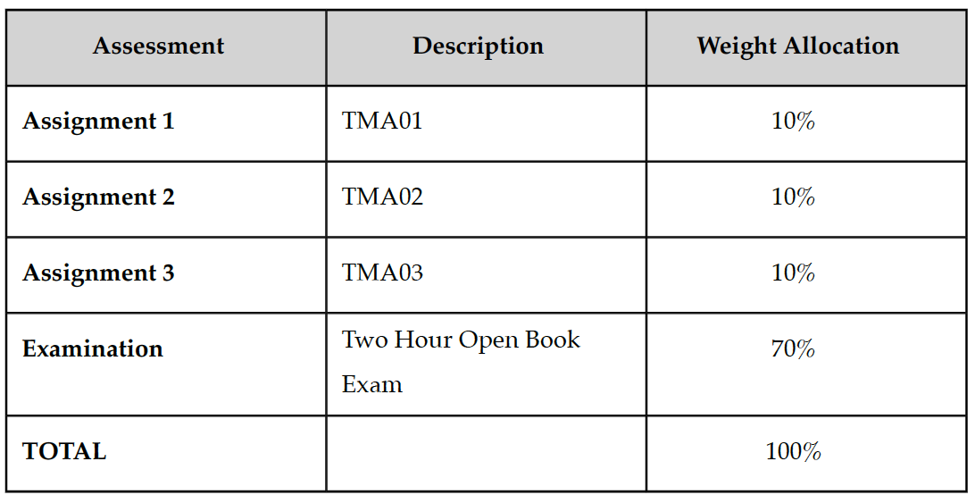
Course Structure
Mar ~ Apr 6 weeks, 6 lectures & 6 labs
Learning Objectives:
- Priority Queue, Binary Heap, Hash Table
- Search Trees: Binary Search Tree, AVL, and Skip List
- Sorting: Insertion Sort, Selection Sort, Bubble Sort, Merge-Sort, Quick Sort
Selection: Prune-and-Search, Randomized-Quicksort - Text Processing: Brute-Force, Boyer-Moore, Knuth-Morris-Pratt and Dynamic Programming
- Graph: Depth-First Search, Breadth-First Search, Dijkstra's Shortest Path, and Min-Spanning Tree
- Review and more
Slides & Notebooks
slides online: https://mth252.fastzhong.com/
https://mth252.fastzhong.com/mth252.pdf
labs: https://github.com/fastzhong/mth252/tree/main/public/notebooks
👉 Python & Big O review: MTH251 lab1
🏃♂️ learning by doing, implementing the algo from scratch
🙇🏻♂️ problem solving


Learning Resource
if you want to dive deeper into proofs and the mathematics of computer science:
📚 Building Blocks for Theoretical Computer Science by Margaret M. Fleck
Clarification
Solution related to DSA questions:
⚠️ always seek the best time and space complexity by appling DSA taught in MTH251 & MTH252
⚠️ in principle, only the standard ADT operations allowed to use by default as the solution has to be language indenpendent
⚠️ advanced features and built-in functions from Python not allowed if not clearly asked by the question, e.g. sort/search/find (in)/min(list)/max(list)/set/match … , as the complexity becomes unknown and Python dependent
Priority Queue
Priority Queue (PQ)
- FIFO/LILO
- each element (k, v) has a certain priority k and k must be compariable
- min priority queue (smaller k, higher priority)
- max priority queue (bigger k, higher priority)
e.g. printer queue, cpu task scheduler, etc.
Priority Queue: Operations
Min PQ
- add(k, v) (enqueue) − adding an element to the queue
- remove_min() (dequeue) − obtain the first element with a pair of (k,v), where k is the mininum value of keys in Min PQ, and remove it from the queue
- min() (first/peek) − obtain the first element with a pair of (k,v) where k is the mininum value of keys in Min PQ
- size(), is_empty()
Max PQ
add(k, v), remove_max(), max(), size(), is_empty()
Priority Queue Complexity
| Operation | unsorted list | sorted list |
|---|---|---|
| is_empty | O(1) | O(1) |
| size | O(1) | O(1) |
| add | O(1) | O(n) 👈 |
| remove_min | O(n) 👈 | O(1) |
| min | O(n) 👈 | O(1) |
Binary Heap
Binary Heap
Complete Binary Tree
k value for any node in the tree smaller than any child node
👉 A perfect binary tree is a tree of which every non-leaf node has two child nodes.
👉 A complete binary tree is a tree in which at every level, except possibly the last is completely filled and all the nodes are as far left as possible.
Binary Heap
key of root is always the smallest (MinHeap) or the largest (MaxHeap)
subtree is also a binary heap
from root to any leaf, the key values are in non-decreasing order
given height h, total nodes of binary heap: 2h≤n≤2h+1−1
given total nodes n, binary heap height: log2(n+1)−1≤h≤log2n
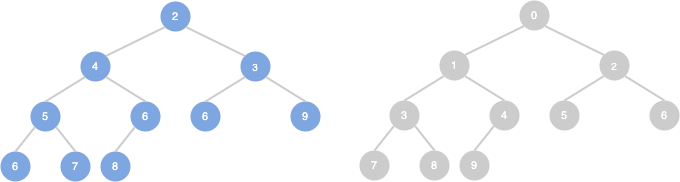
Binary Heap
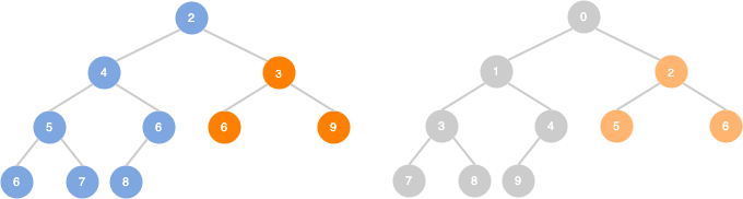
| 2 | 4 | 3 | 5 | 6 | 6 | 9 | 6 | 7 | 8 |
| 0 | 1 | 2 | 3 | 4 | 5 | 6 | 7 | 8 | 9 |
| current node | : | i |
| parent(i) | = | (i - 1) / 2 |
| left_child(i) | = | 2 * i + 1 |
| right_child(i) | = | 2 * i + 2 |
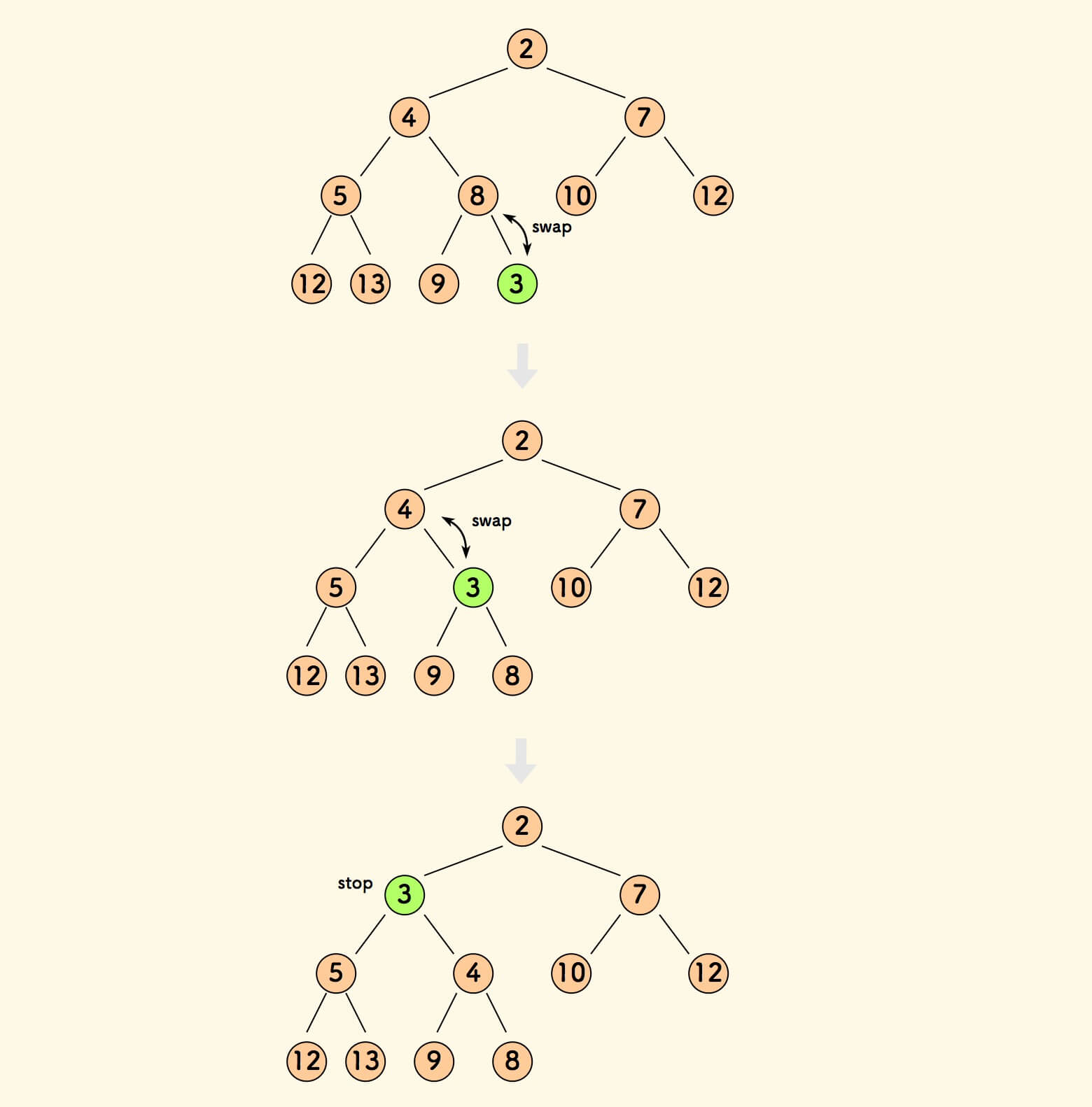
Binary Heap
add new element:
- append to the last (so its still complete binary tree)
- sift up if new element is smaller
Binary Heap
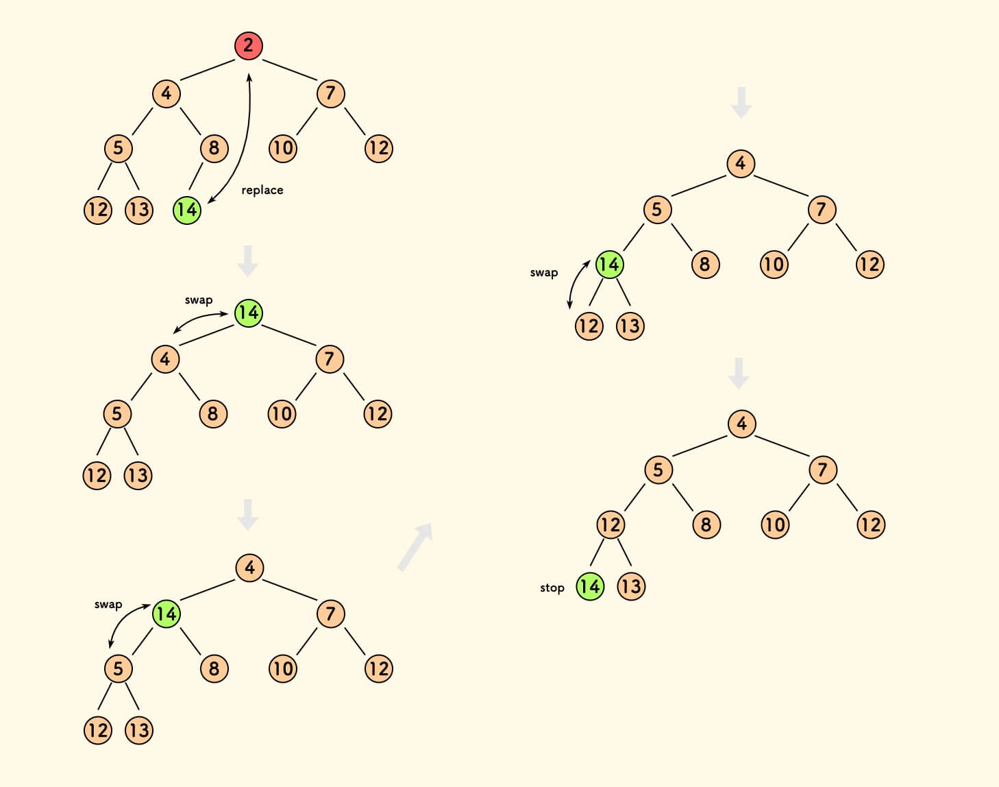
remove the min:
- replace the first element with the last (so its still complete binary tree)
- sift down if the last element is bigger
Priority Queue Complexity
| Operation | unsorted list | sorted list | binary heap |
|---|---|---|---|
| is_empty | O(1) | O(1) | O(1) |
| size | O(1) | O(1) | O(1) |
| add | O(1) | O(n) | O(logN) 👈 |
| remove_min | O(n) | O(1) | O(logN) 👈 |
| min | O(n) | O(1) | O(1) |
When & Where
Priority Queue (PQ) is used:
used in certain implementations of Dijkstra’s Shortest Path algorithm
used by Minimum Spanning Tree (MST) algorithms
Best First Search (BFS) algorithms such as A* uses PQ to continuously grab the next most promising node
used in Huffman coding (which is often used for lossless data compression)
anytime you need to dynamically fetch the "next best" or "next worst" element
…
Heap Sort
Steps:
create a binary heap
add all elements to the heap
recursively obtain the min/max element from the heap
# heap sort

# time complexity: O(NlogN)
# space complexity: O(N)
def heap_sort(nums: []) -> []:
    if not nums:
        return []
    minH = MinHeap()
    for e in nums:
        minH.add((e, e))
    nums_sorted = []
    for i in range(len(nums)):
        nums[i] = minH.remove_min()[0]
    return nums# heap sort

# time complexity: O(NlogN)
# space complexity: O(N)
def heap_sort(nums: []) -> []:
    if not nums:
        return []
    minH = MinHeap()
    for e in nums:
        minH.add((e, e))
    nums_sorted = []
    for i in range(len(nums)):
        nums[i] = minH.remove_min()[0]
    return nums
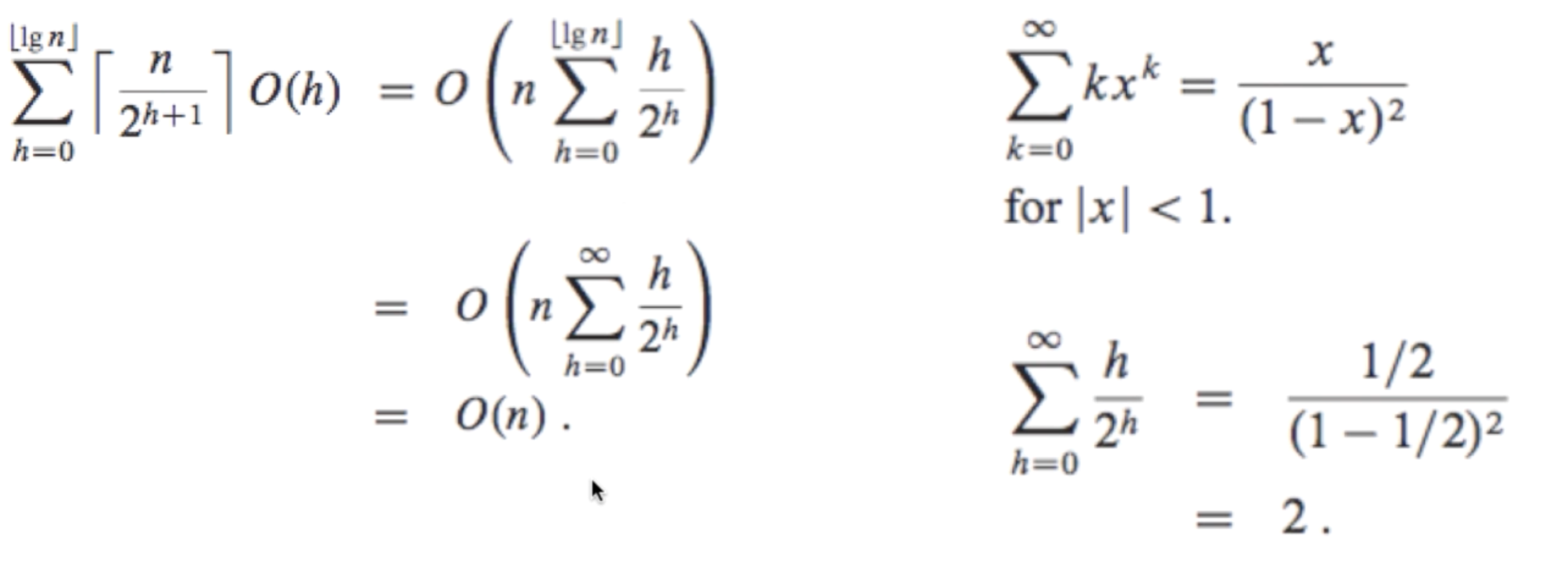
Heapify
Heapify: convert the array to be a binary heap
by "sift down" the non-leaf node one by one from top to bottom
Complete Binary Tree (Perfect Binary Tree in worst case)
| last level nodes: | 2n | sift_down: | 2n∗0 |
| 2nd last level nodes: | 4n | sift_down: | 4n∗1 |
| … | … | ||
| h+1 last level nodes: | 2h+1n | sift_down: | 2h+1n⋅h |
Time Complexity: O(n)
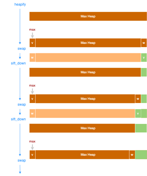
Heap Sort
"""
heap_sort: sort nums in place

time complexity: O(N)
space complexity: O(1)
"""
def heap_sort2(nums: []) -> []:
    nums = heapify(nums)
    print("    heapify: ", nums)
    # swap from the last element
    for i in range(len(nums) - 1, 0, -1):
        # move the biggest to the end
        nums[0], nums[i] = nums[i], nums[0]
        # sift down the first element after swap
        # so nums[0, i) is still a max heap
        heapify_sift_down(nums, 0, i)
    return nums"""
heap_sort: sort nums in place

time complexity: O(N)
space complexity: O(1)
"""
def heap_sort2(nums: []) -> []:
    nums = heapify(nums)
    print("    heapify: ", nums)
    # swap from the last element
    for i in range(len(nums) - 1, 0, -1):
        # move the biggest to the end
        nums[0], nums[i] = nums[i], nums[0]
        # sift down the first element after swap
        # so nums[0, i) is still a max heap
        heapify_sift_down(nums, 0, i)
    return nums
Map/Hash Table
Map
A Map is an abstract data structure (ADT):
- a collection of key-value (k,v) paris
- key can be viewed as a unique identifier for the object/value
k - unique
v - can be repeated
A Sorted Map is an extension of Map and keys are sorted in increasing order.
🤔 Can we use none/null for key?
Map
students score:
| Student(key) | Score(value) |
|---|---|
| A | 80 |
| B | 70 |
| C | 60 |
| … | … |
Map Operations
for a map
- map[k], map.get(k)
- map.pop(k)
- map[k] = v, map.set(k) = v, map.put(k,v), map.setdefault(k, default)
- map.keys()
- map.values()
- del map[k], map.clear()
- size(map)
- iter(map), map.items()
Map Operations
for a sortedMap
- sortedMap.find_min()
- sortedMap.find_max()
- sortedMap.find_lt(k)
- sortedMap.find_le(k)
- sortedMap.find_gt(k)
- sortedMap.find_ge(k)
- sortedMap.find_range(k1, k2)
- sortedMap.reversed()
Map Implementation
- Array/ArrayList
- Linked List
- Binary Search Tree
- Hash Table
- Skip List
Map Implementation: Linked List
- store (k,v) in a doubly linked list
- get(k)
- loop through the list until find the element with key k
- set(k,v)
- create a new node (k,v) and add it at the front
- delete(k)
- loop through the list until find the element with key k
- remove it by updating the pre and next elements
👉 Complexity: O(n)
Hash Table
A Hash table is a data structure that provides a mapping from keys to values using a technique called hashing.
A hash function H(x) is a function that maps a general key ‘x’ to a whole number in a fixed range [0, N-1].
💡 locate the element without searching: O(n) → O(1)
Hash Function
step1. Hash Code: abitrary object → integer
An element is converted into an integer by using a hash function. This element can be used as an index to store the original element, which falls into the hash table.
hash = hashcode(key)hash = hashcode(key)
step2. Compression: integer∈[0,N−1] (N is the size of hash table)
The element is stored in the hash table where it can be quickly retrieved using hashed key.
index = hash % array_sizeindex = hash % array_size
Hash Code: Bit Representation
# XOR byte by byte
def byte_xor(ba1, ba2):
    return bytes([_a ^ _b for _a, _b in zip(ba1, ba2)])

# produce 32-byte hash code
# chop the data into 32-byte long chunks (padding with zeros if required)
# then XOR on all chunks
def bitwise_xor(data):
    chunks = [data[i:i+32] for i in range(0, len(data), 32)]
    for i in range(len(chunks)):
        chunk = chunks[i]
        hexchunk = chunk.hex()
        len_diff = 32 - len(chunk)
        if len_diff:
            hexchunk += '00' * len_diff
            chunk = bytearray.fromhex(hexchunk)
            chunks[i] = chunk
    res = bytes.fromhex('00' * 32)
    for chunk in chunks:
        res = byte_xor(res, chunk)
    return res# XOR byte by byte
def byte_xor(ba1, ba2):
    return bytes([_a ^ _b for _a, _b in zip(ba1, ba2)])

# produce 32-byte hash code
# chop the data into 32-byte long chunks (padding with zeros if required)
# then XOR on all chunks
def bitwise_xor(data):
    chunks = [data[i:i+32] for i in range(0, len(data), 32)]
    for i in range(len(chunks)):
        chunk = chunks[i]
        hexchunk = chunk.hex()
        len_diff = 32 - len(chunk)
        if len_diff:
            hexchunk += '00' * len_diff
            chunk = bytearray.fromhex(hexchunk)
            chunks[i] = chunk
    res = bytes.fromhex('00' * 32)
    for chunk in chunks:
        res = byte_xor(res, chunk)
    return res
Hash Code: Polynomial & Cyclic-Shift
Polynomial
for n-tuple (x0,x1,x2,...,xn−1), if position is important, we can multiply an−1 for position n, e.g.:
x0⋅a0+x1⋅a1+x2⋅a2+...+xn−1⋅an−1
Cyclic-Shift
for bitwise, we can also apply cyclic-shift function instead of multiplication, e.g. shift(x, y) means cyclic-shift y bits:
shift(x0,0mod32)⊕shift(x1,1mod32)⊕shift(x2,2mod32)⊕...⊕shift(xn−1,(n−1)mod32)
💬 5-bit cyclic shift operation can achieve the smallest total collisions when 230,000 English words
Hash Function: Compression
for hash code x:
Division Method: xmodN
MAD: (a⋅x+b)modp where p is a prime number, p>N, a and b are random number, a∈[0,p−1], b∈[0,p−1]
Hash Function
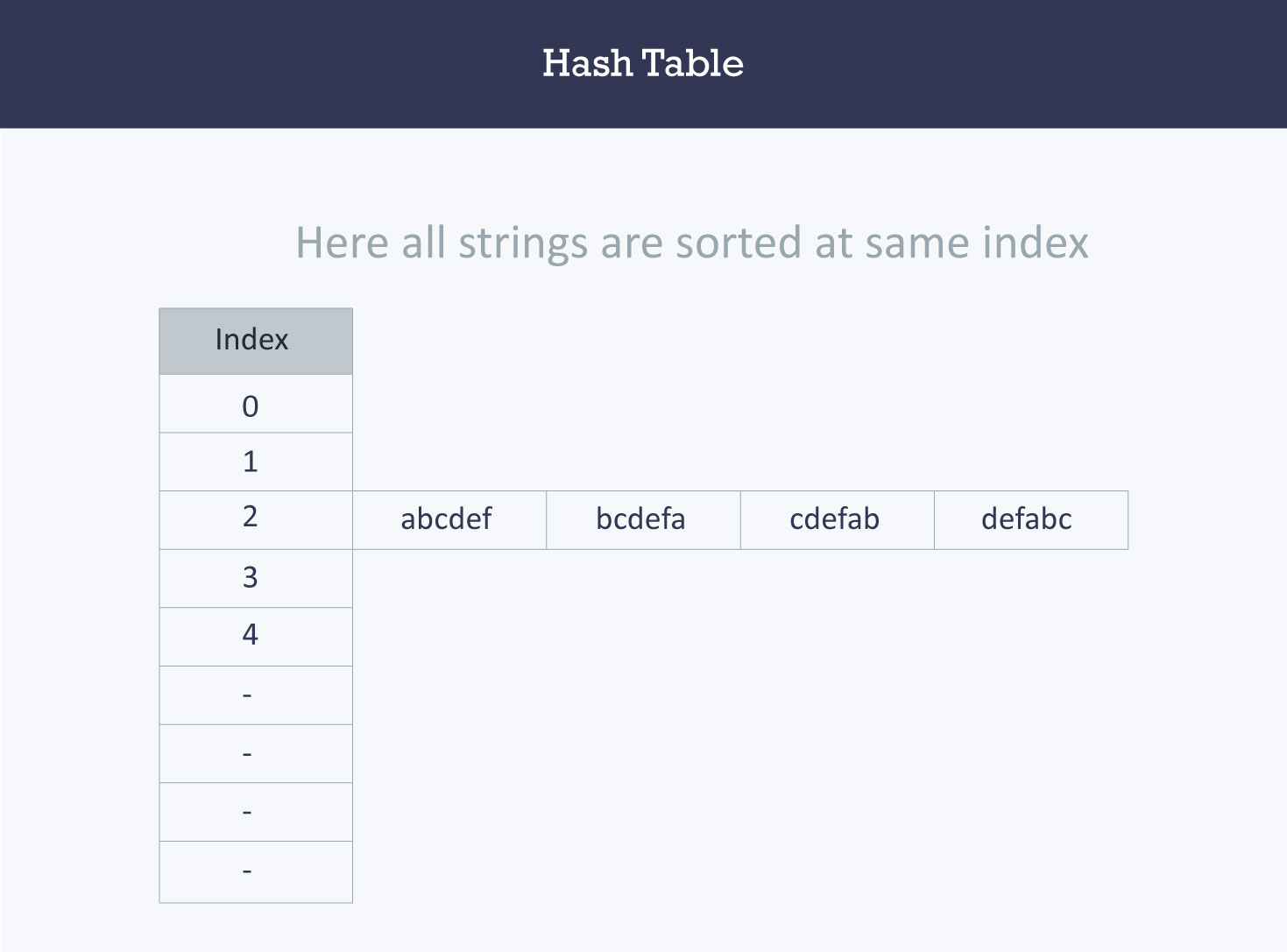
a number of (k, v) pairs with key set {“abcdef”, “bcdefa”, “cdefab” , “defabc”}
The ASCII values of a, b, c, d, e, and f are 97, 98, 99, 100, 101, and 102 respectively.
| key | Hash Function | Index |
|---|---|---|
| abcdef | (97 + 98 + 99 + 100 + 101 + 102) % 599 | 2 |
| bcdefa | (98 + 99 + 100 + 101 + 102 + 97) % 599 | 2 |
| cdefab | (99 + 100 + 101 + 102 + 97 + 98) % 599 | 2 |
| defabc | (100 + 101 + 102 + 97 + 98 + 99) % 599 | 2 |
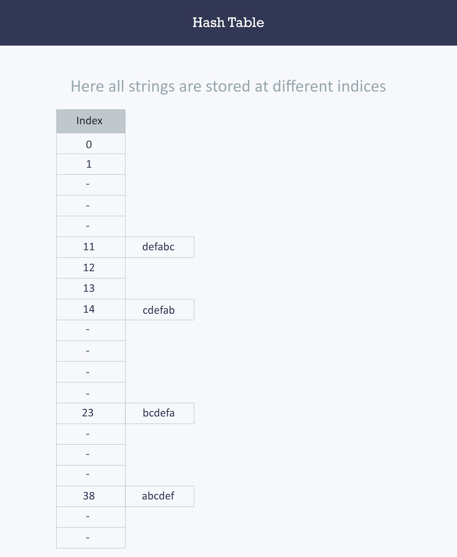
Hash Function
a number of (k, v) with key set {“abcdef”, “bcdefa”, “cdefab” , “defabc”}
The ASCII values of a, b, c, d, e, and f are 97, 98, 99, 100, 101, and 102 respectively.
| key | Hash Function | Index |
|---|---|---|
| abcdef | (971 + 982 + 993 + 1004 + 1015 + 1026) % 2069 | 38 |
| bcdefa | (981 + 992 + 1003 + 1014 + 1025 + 976) % 2069 | 23 |
| cdefab | (991 + 1002 + 1013 + 1024 + 975 + 986) % 2069 | 14 |
| defabc | (1001 + 1012 + 1023 + 974 + 985 + 996) % 2069 | 11 |
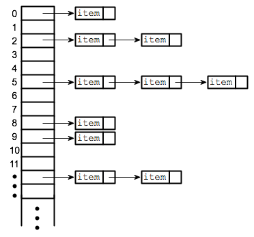
Hash Function: Collision
chaining (open hashing)
one element: O(1)
more than one element: linked list O(1)+O(n)
Hash Function: Collision
open address (closed hashing)
Finding an unused, or open, location in the hash table is called open addressing.
The process of locating an open location in the hash table is called probing.
Various probing techniques:

index = (index + 1) % hashTableSize
index = (index + 2) % hashTableSize
index = (index + 3) % hashTableSize
...

index = (index + 1^2) % hashTableSize
index = (index + 2^2) % hashTableSize
index = (index + 3^2) % hashTableSize
...

index = (index + 1 * H2) % hashTableSize
index = (index + 2 * H2) % hashTableSize
index = (index + 3 * H2) % hashTableSize
...
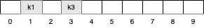
Hash Function: Collision
⚠️ probing may go into cycles (an infinite loop) (hashing attack)
⚠️ chaos when removing element from hash table
- put(k2,v2) (probing: 1 → 2)
- put(k3,v3) (probing: 1 → 2 → 3)
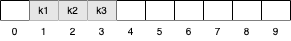
- get(k3) (probing: 1 → 2)
Hash Table: resize
M: total num of map elements
O: num of occupied buckets
N: size of hash table
P: new size of hash table (expand or shrink)
when:
- load factor (for open addressing): NO
- tolerance factor (for closed addressing): NM
how:
- size(good hash table primes): N → P
- rehashing: H(x)modN → H(x)modP
Hash Function
H(x):
- deterministic
- fast as O(1)
- universal input
- evenly distributed
- randomly distributed
Designing good hash functions requires a blending of sophisticated mathematics and clever engineering.
Hash Function
- if x=y, H(x) and H(y) must be equal
- if H(x)=H(y), x and y might be equal
- if H(x)=H(y), x and y certainly not equal
💡 coding tips:
- avoid to use real or big number as key: H(0.0)==H(−0.0) ?
- compare hash code first, before compare x and y
- overwrite either both of eq and hash or neither of them
class UserGroup:

  def __init__(self, name, status):
    self.name = name
    self.status = status

  def __hash__(self):
    result = 17
    result = 31 * result + hash(name)
    if not status:
      result = 31 * result + hash(status)
    return result

  def __eq__(self, other):
    if isinstance(other, UserGroup):
      return self.__hash__() == other.__hash__()
    return Falseclass UserGroup:

  def __init__(self, name, status):
    self.name = name
    self.status = status

  def __hash__(self):
    result = 17
    result = 31 * result + hash(name)
    if not status:
      result = 31 * result + hash(status)
    return result

  def __eq__(self, other):
    if isinstance(other, UserGroup):
      return self.__hash__() == other.__hash__()
    return False
Map/Hash Table Complexity
| Operation | avg case | best case | worst case |
|---|---|---|---|
| Search | O(1) | O(1) | O(n) |
| Insert | O(1) | O(1) | O(n) |
| Delete | O(1) | O(1) | O(n) |
Industrial Implementation
HashMap
- hash code
| Key Type | hashCode(k) |
| boolean | k? 0 : 1 |
| byte, char, short, int | k |
| long | (int)(k XOR (k >>> 32)) |
| float | Float.floatToIntBits(k) |
| double | long l = Double.doubleToIntLongBits(k) (int)(l XOR (l >>> 32)) |
| string/array | s[0]*31^(n-1) + s[1]*31^(n-2)+ ... + s[n-1] |
similarly for compound data type, like Object k with n fields, a way to implement hashCode():
h=h(k0)∗31n−1+h(k1)∗31n−2+...+h(kn−1)
String name;
int age;

@Override
public int hashCode() {
    int result = name != null ? name.hashCode() : 0;
    result = 31 * result + age;
    return result;
}String name;
int age;

@Override
public int hashCode() {
    int result = name != null ? name.hashCode() : 0;
    result = 31 * result + age;
    return result;
}
Industrial Implementation
HashMap
- compression/indexing: h&(n−1)
when table size n is 2y: x%2y=x&(y−1)
e.g.
6%8=6 6&7=610%8=2 10&7=2
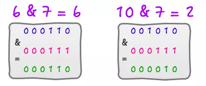
👉 binary bit operation & is much faster then decimal mod
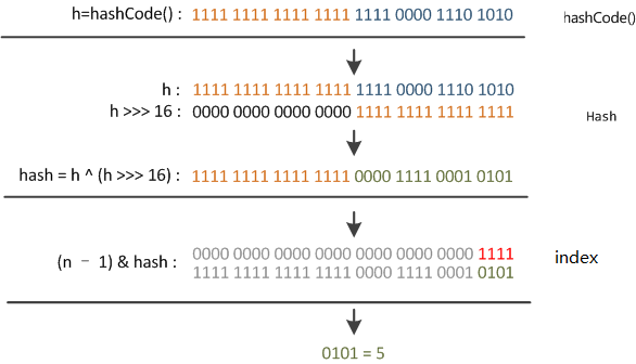
then XOR between the first 16 bits and the last 16 bits:
H(k)=(hXOR(h>>>16))&(n−1)
Industrial Implementation
HashMap
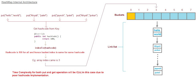
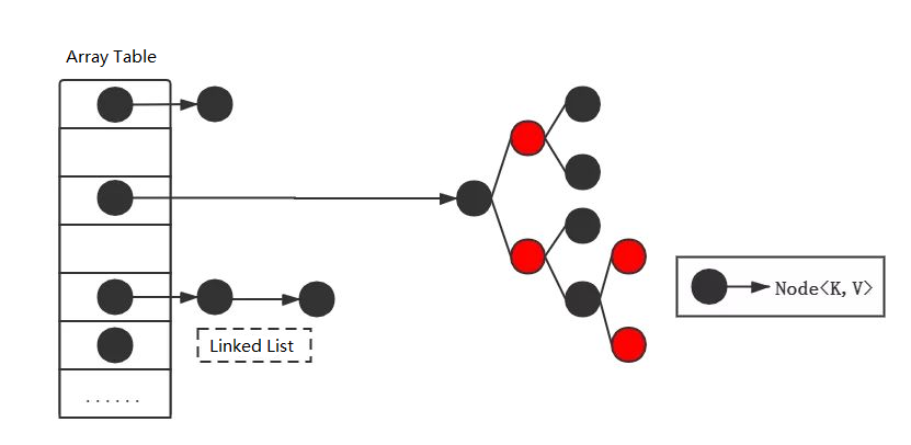
- Collision: chaining
- linked list O(1)+O(n)
- <Java8, insert at the beginneing (⚠️ deadlock in concurrent insertion); >Java8, append to the tail
- treemap/red black tree (more than 8 elements and table size ≧ 64) O(1)+O(logN)
Industrial Implementation
HashMap
- hash table size
- always 2n, default: 16, max: 230
- load factor: 0.75
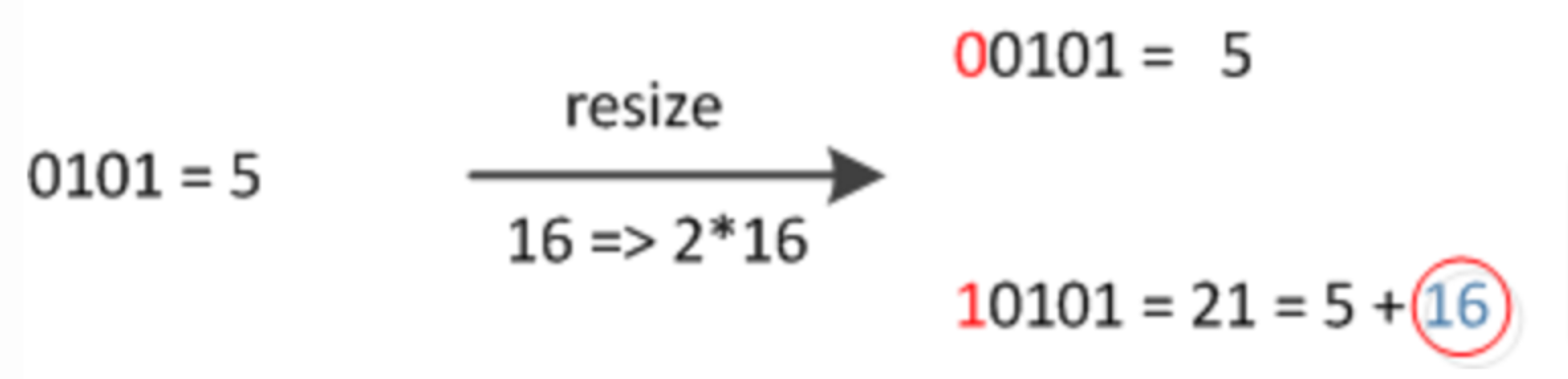
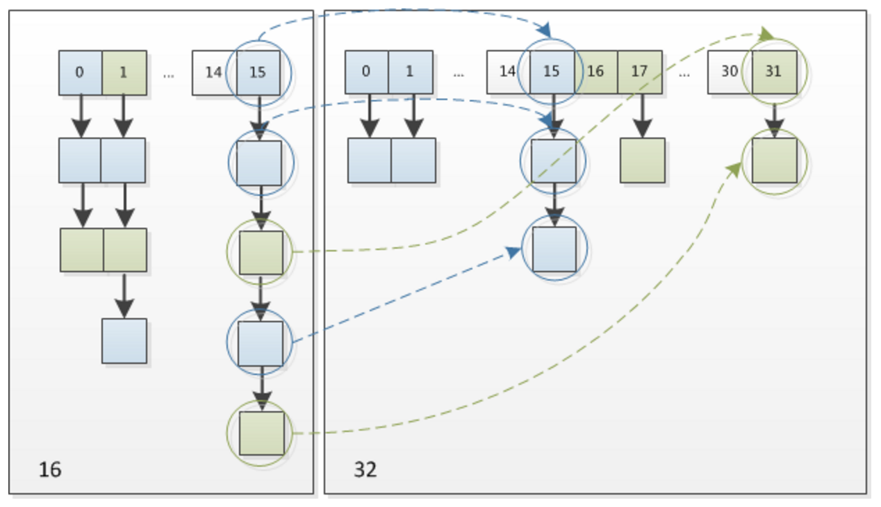
- optimize rehashing
size 16 → 16∗2:
Industrial Implementation
HashMap
- HashMap for HashSet: HashSet<E> → HashMap<E, Object>
- {e1, e2, e3, …} → (e1, PRESENT), (e2, PRESENT), (e3, PRESENT), …
👉 source code: https://github.com/frohoff/jdk8u-jdk/blob/master/src/share/classes/java/util/HashMap.java
Binary Search Tree
Binary Search Tree (BST)
Binary Search Tree (BST) is a binary tree and:
- left subtree has smaller elements
- right subtree has bigger elements
💡 any BST subtree is still a BST
💡 BST node must be comparable
💬 in some BST implementation all values are unique, so we exclude duplicates now
BST: Operations
- search()
- insert()
- delete()
- first()
- last()
- before()
- after()
- is_empty()
💬 1962, Hibbard Deletion
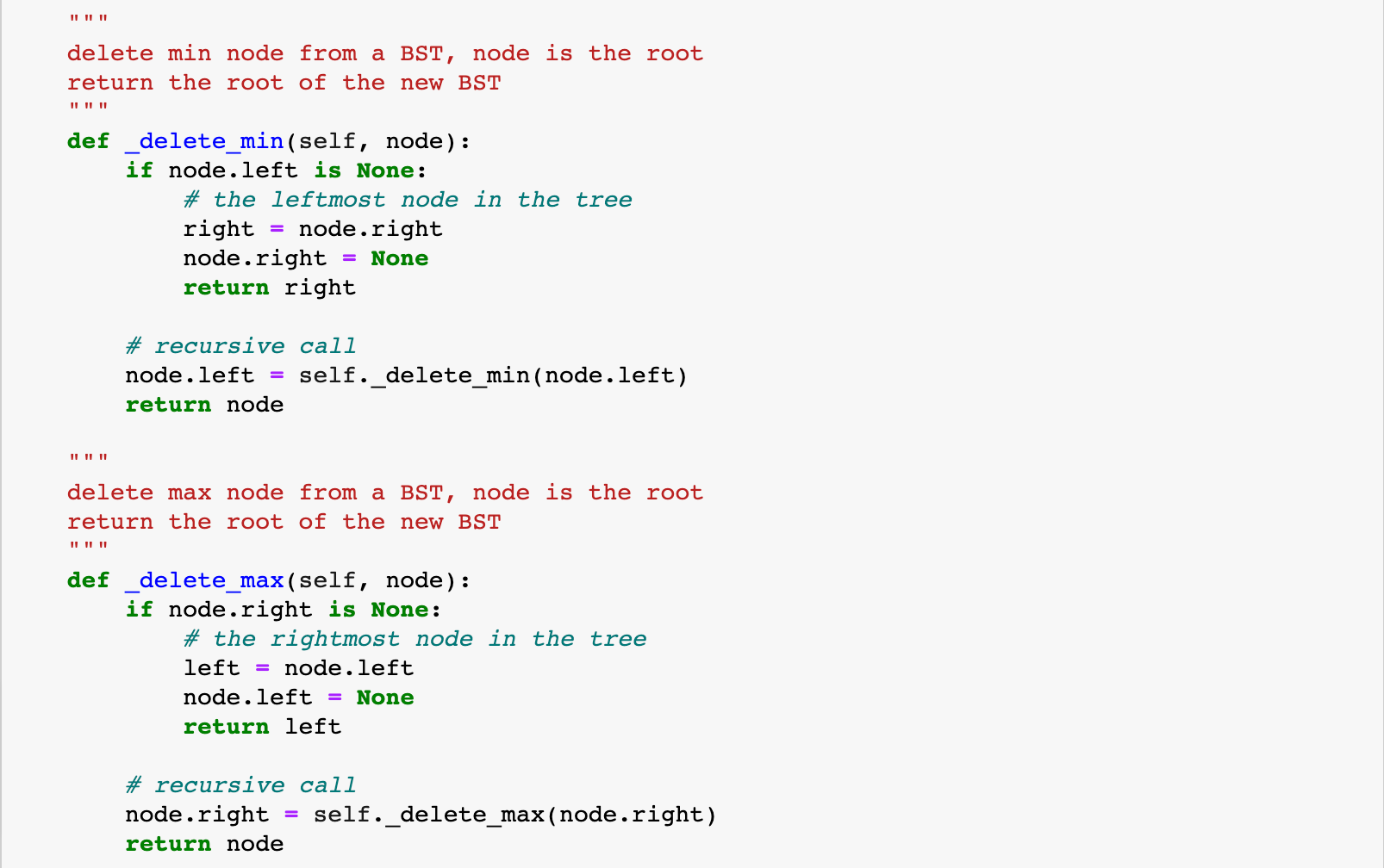
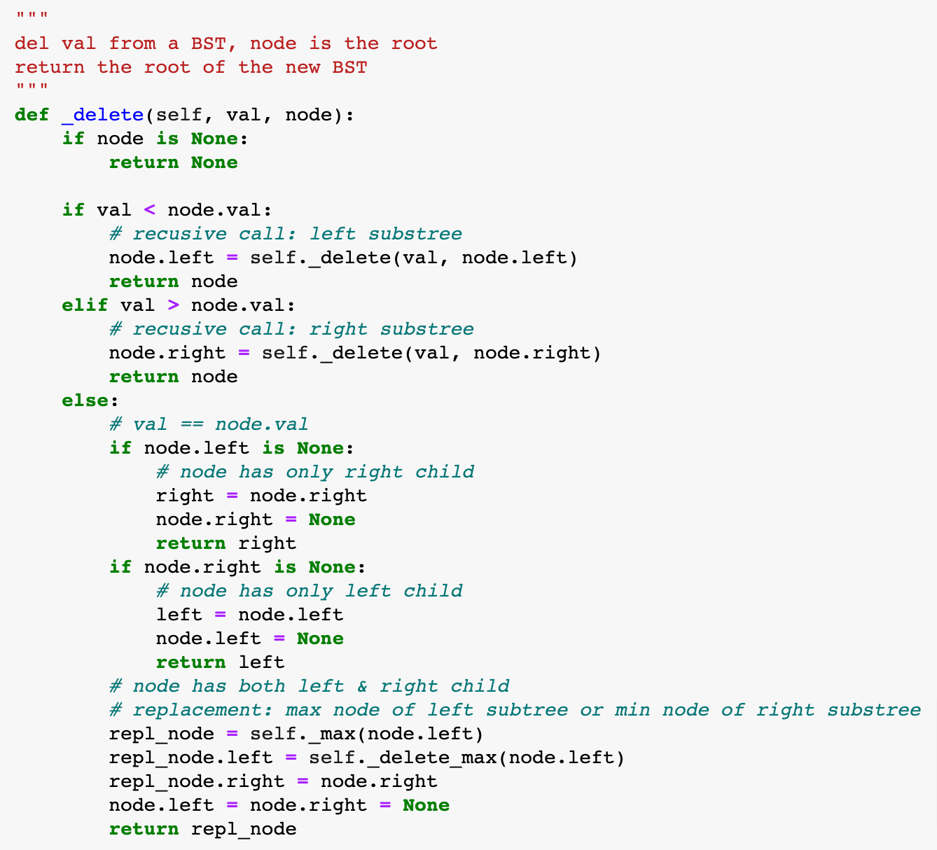
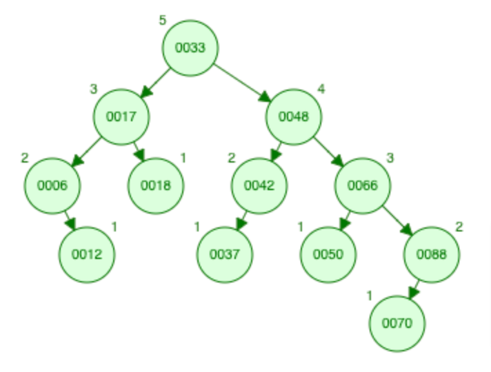
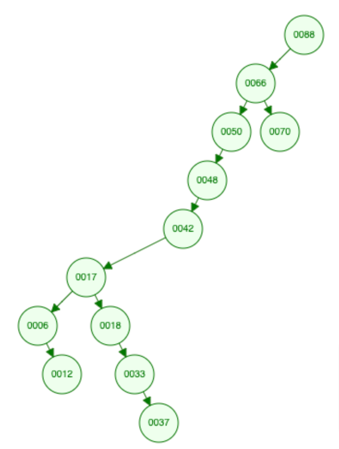
BST: Hibbard Deletion
del min
del max
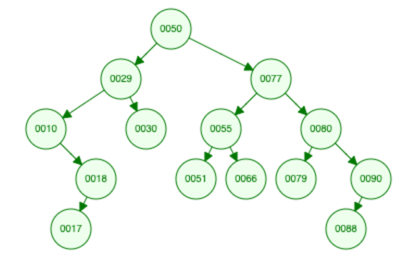
BST: Hibbard Deletion
del 10
"node with 1 child node"
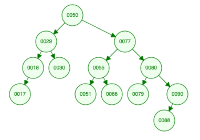
BST: Hibbard Deletion
del 77
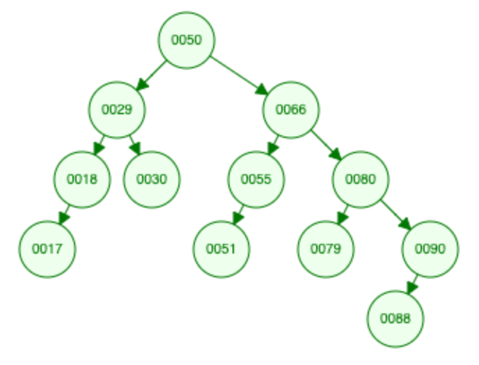
"node with 2 child nodes"
BST: Traversal
- pre-order
- in-order: "sorted list" 👈
- post-order
- level order
Binary Search Tree Complexity
| Operation | avg case | worst case |
|---|---|---|
| Search | O(logN) | O(n) |
| Insert | O(logN) | O(n) |
| Delete | O(logN) | O(n) |
When & Where
Binary Search Tree (BST) is used:
implementation of AVL Tree Red Black Tree etc.
syntax trees used by compiler and calculator
Treap - a probabilistic data structure
…
BST vs Heap
Heap is balanced tree, BST is not
Heap allows duplicates, BST doesnot
BST is ordered data structure, Heap is not
worst case for building n nodes of BST O(n⋅log(n)), Heap is O(n) (heapify)
AVL
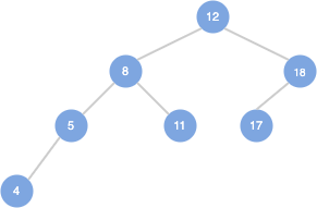
AVL
named after inventors G.M. Adel’son-Vel’skii and E.M. Landis, 1962
first type of Balanced Binary Search Tree (BBST)
height balanced: BF - balance factor
BF=H(node.right)−H(node.left)
BF∈−1,0,1heigh and no. of nodes: O(logN)
Examples:
- perfect binary tree (minimum heigh)
- complete binary tree
- Binary Heap, Red Black Tree, Segment Tree, etc.
AVL Balance Factor
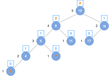
Rebalance ?
- When: insert(), delete()
- Where: backtracking from the node
AVL insert & delete
Steps:
update Height
compute Balance Factor
left/right rotation if unbalanced
👉 https://www.cs.usfca.edu/~galles/visualization/AVLtree.html
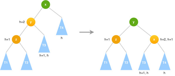
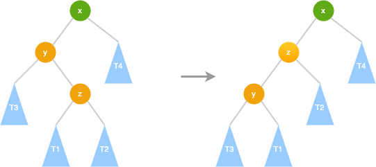
AVL Right Rotate (LL)
T1<z<T2<y<T3<z<T4
-   y.right = x
-   x.left = T3-   y.right = x
-   x.left = T3
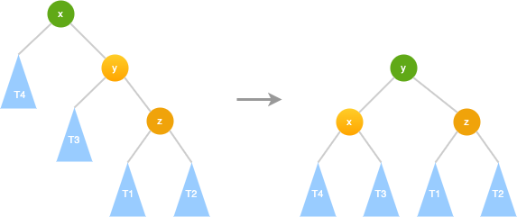
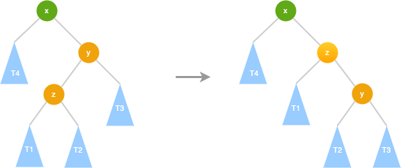
AVL Left Rotate (RR)
T4<x<T3<y<T1<z<T2
-   y.left = x
-   x.right = T3-   y.left = x
-   x.right = T3
AVL LR → LL
1. LR → LL: left rotate
2. LL: right rotate1. LR → LL: left rotate
2. LL: right rotate
AVL RL → RR
1. RL → RR: right rotate
2. RR: left rotate1. RL → RR: right rotate
2. RR: left rotate
BST vs AVL Complexity
| Operation | BST avg | BST worst | AVL avg | AVL worst |
|---|---|---|---|---|
| Search | O(logN) | O(N) | O(logN) | O(logN) |
| Insert | O(logN) | O(N) | O(logN) | O(logN) |
| Delete | O(logN) | O(N) | O(logN) | O(logN) |
AVL: O(N) → O(logN)
Red Black Tree
Red Black Tree
A red-black tree is a binary tree that satisfies the following red-black properties:
- every node is either red or black
- the root is black
- every leaf (NIL) is black
- if a node is red, both its children are black
- for each node, all simple paths from the node to descendant leaves contain the same number of black nodes
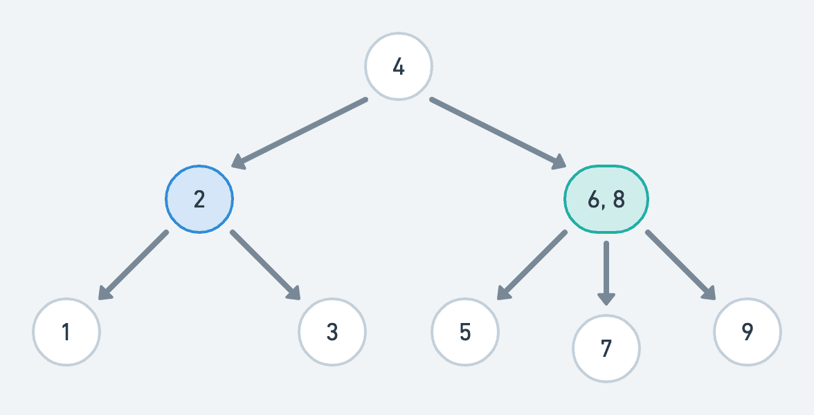
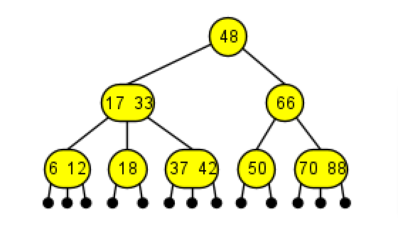
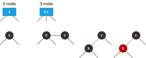
2-3 Tree
A 2-3 tree is a B-tree of order 3:
- 2-node: node with two child nodes
- 3-node: node with three child nodes
- a perfectly balanced tree: all leaf nodes at the same level


2-3 Tree
Insertion is always done on leaf
- merge: insert into a node with only data element (2-node leaf)
- merge & split: insert into a node with two data element (3-node leaf) whose parent contains only one data element (2-node parent)
- merge⁺⁺ & split⁺⁺ : insert into a node with two data element (3-node leaf) whose parent contains two data element (3-node parent)
Red Black Tree
Red Black Tree is equivalent 2-3 Tree
Red Black Tree
Red Black Tree is equivalent 2-3 Tree
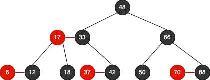
"black balanced"
N nodes → height: 2logN, Complexity: O(logN)
Red Black Tree vs AVL Tree
Red Black Tree
insert a red node → a blank tree
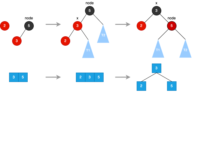
Red Black Tree
Left Rotate
-   node.right = x.left
-   x.left = node
-   x.color = node.color
-   node.color = RED-   node.right = x.left
-   x.left = node
-   x.color = node.color
-   node.color = RED
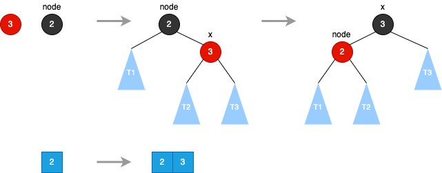
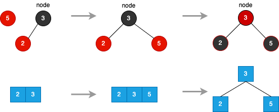
Red Black Tree
Flip Colors
-   node.color = RED
-   node.left.color = BLACK
-   node.right.color = BLACK-   node.color = RED
-   node.left.color = BLACK
-   node.right.color = BLACK
Red Black Tree
Right Rotate
-   node.left = T1
-   x.right = node
-   x.color = node.color
-   node.color = RED-   node.left = T1
-   x.right = node
-   x.color = node.color
-   node.color = RED
Red Black Tree
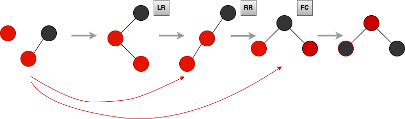
insertion: LR → RR → FC
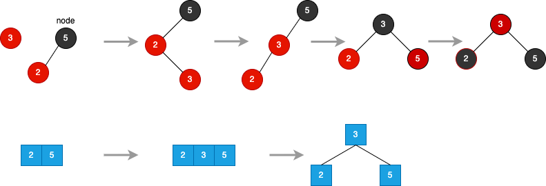
Red Black Tree
insertion: LR → RR → FC
- 2-node
- 3-node
Skip List
Skip List
Skip List
search key
Skip List
delete key
Skip List
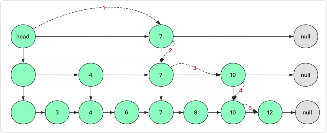
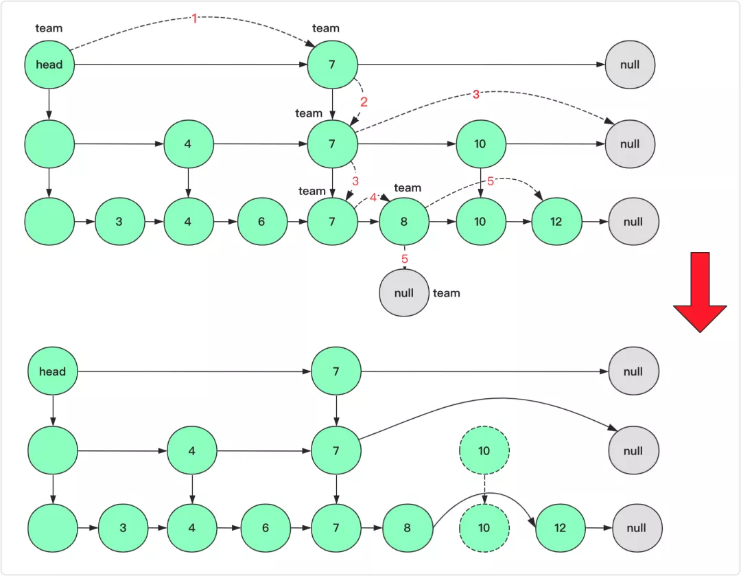
insert key
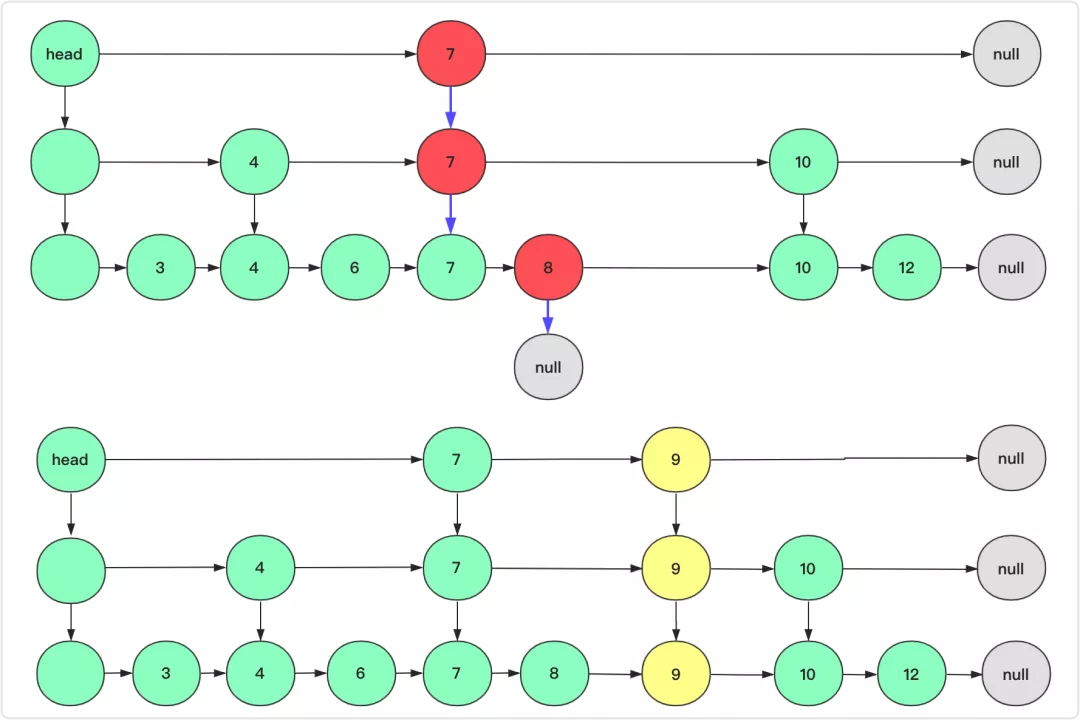
Skip List
insert key
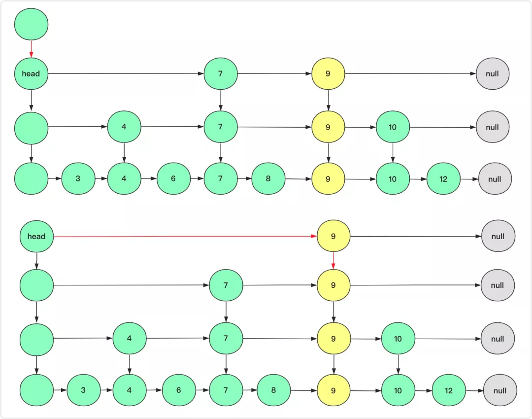
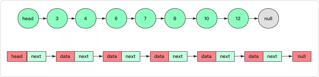
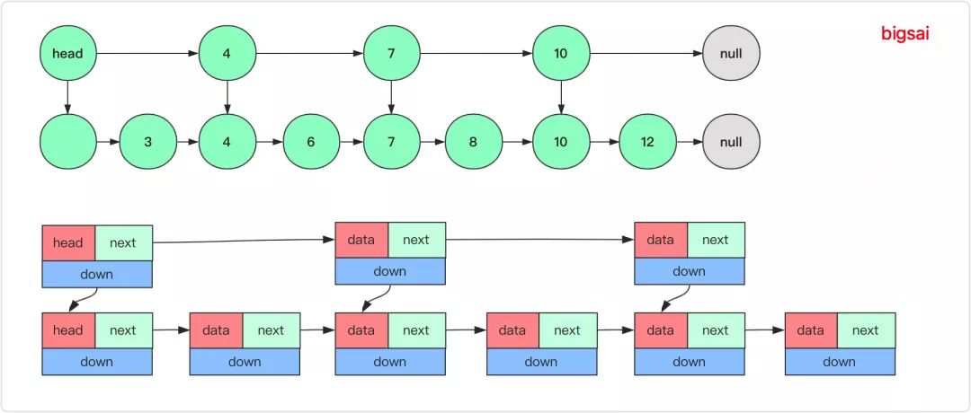
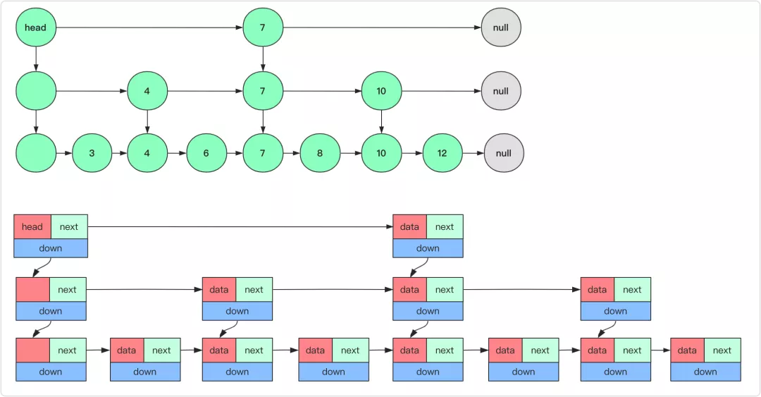
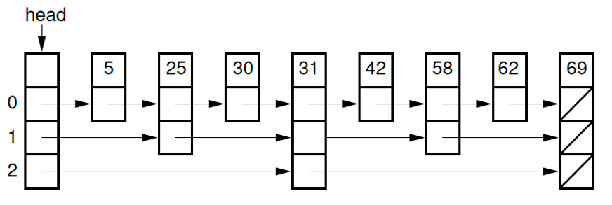
Skip List
Skip List node with an array of pointers: position pointers[0] stores a level 0 pointer, position pointers[1] stores a level 1 pointer, and so on.
When inserting a new value, the levels (depth) for the new node is randomized.
Skip List Complexity
| Operation | Skip List avg | Link List avg |
|---|---|---|
| Search | O(logN) 👈 | O(N) |
| Insert | O(logN) | O(N) |
| Delete | O(logN) | O(N) |
👉 Skip Lists: A Probabilistic Alternative to Balanced Trees (William Pugh, 1990)
Skip List vs Hash Table, Balanced Tree
- single key search, Hash Table close to O(1)
- for Skip List node, avg no. of pointers 1−pp, when p=41, 1.33<2
- keys in order, better for range search
- Skip List operations (linkedlist++) simpler than balanced tree (AVL, Red Black Tree, etc.)
- Skip List overall implementation simpler
Sorting
Sorting
- make data in order
- different algorithmic thinking
Sorting: Selection
- sort the arr from left to right
- every time select the smallest
- for position i:
- [0,i) sorted
- [i,n) unsorted
- find the smallest from arr[i,n) and place at arr[i]
- Complexity: 1+2+3+...+n=2(n+1)∗n
Sorting: Insertion
- sort the arr from left to right
- for postion i:
- [0,i) sorted
- [i,n) unsorted
- insert arr[i] to the proper position on the left
- Complexity: O(n2), if already sorted → O(n) 👍
Sorting: Bubble
- sort the arr from right to left
- for postion n−i−1:
- [n−i,n) sorted
- [0,n−i−1) unsorted
- bubble the biggest to arr[n−i−1]
- Complexity: O(n2)
Sorting: Merge
John von Neumann
- recursively [l,m,r]:
- sort [l,m]
- sort [m+1,r]
- merge two sorted array [l,m] & [m+1,r]

Sorting: Merge
merge top down: sort_merge_bottomup_v1
improvement: sort_merge_recusive_v2- ✅ insertion
- ❌ tmp
merge buttom up: sort_merge_bottomup
worst case ?
- almost sorted array
- duplicates
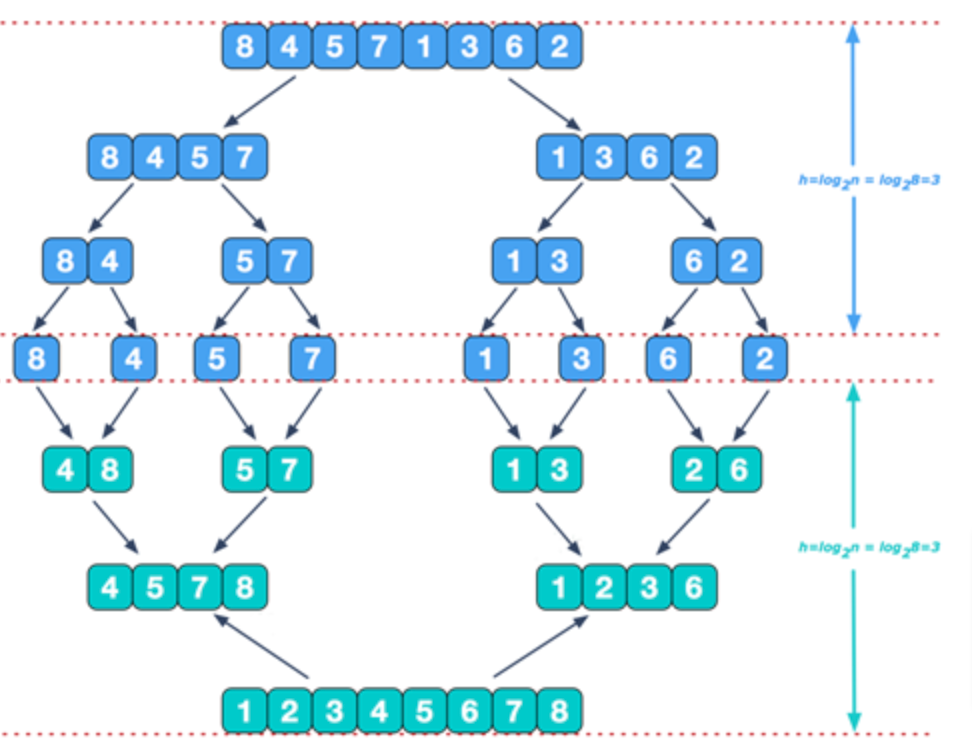
Sorting: Merge
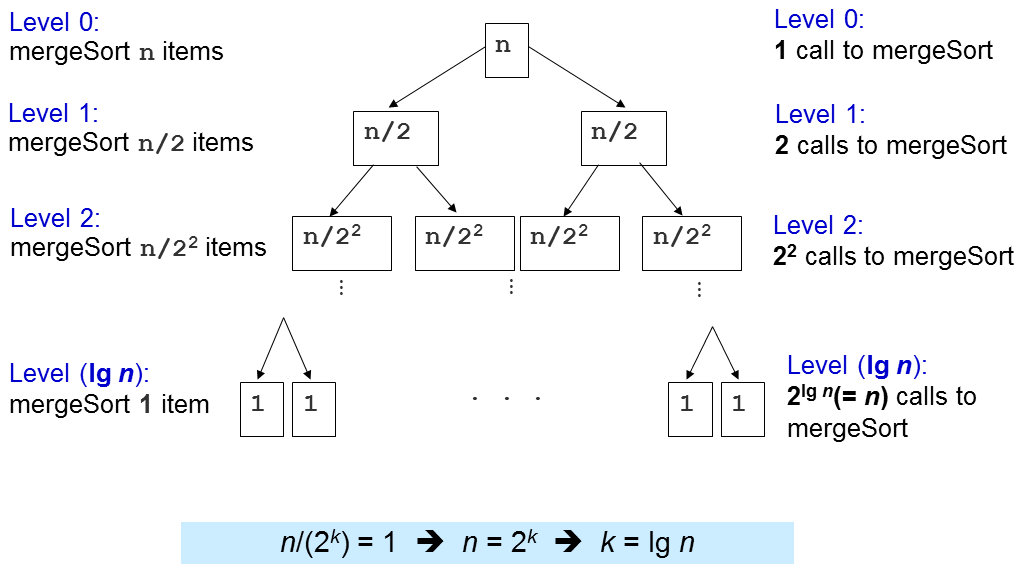
- Time Complexity O(n⋅log2n)
- Space Complexity O(n)
at each level i = 0,1,2,...,log2n
there are 2i subproblems, each of size 2in
total # of operations at level i ≤2i⋅c(2in)=c⋅n
complexity on each level is O(n)
"recursion tree"
Sorting: Quick
Tony Hoare

- partition: select v, so that [l,p−1]≤v and [p+1,r]≥v
- recursive sort [l,p−1]
- recursive sort [p+1,r]
Sorting: Quick
worst case: O(n2)
- sorted array
- duplicates
- O(n2) possibility: n1∗n−11∗n−21∗...=n!1
- recusion stack overflow
improvement:
- 2-way quicksort
- 3-way quicksort
- dual pivot quicksort
👉 random algorithm, time complexity O(N⋅log2N) (📚 Introduction to Algorithms)
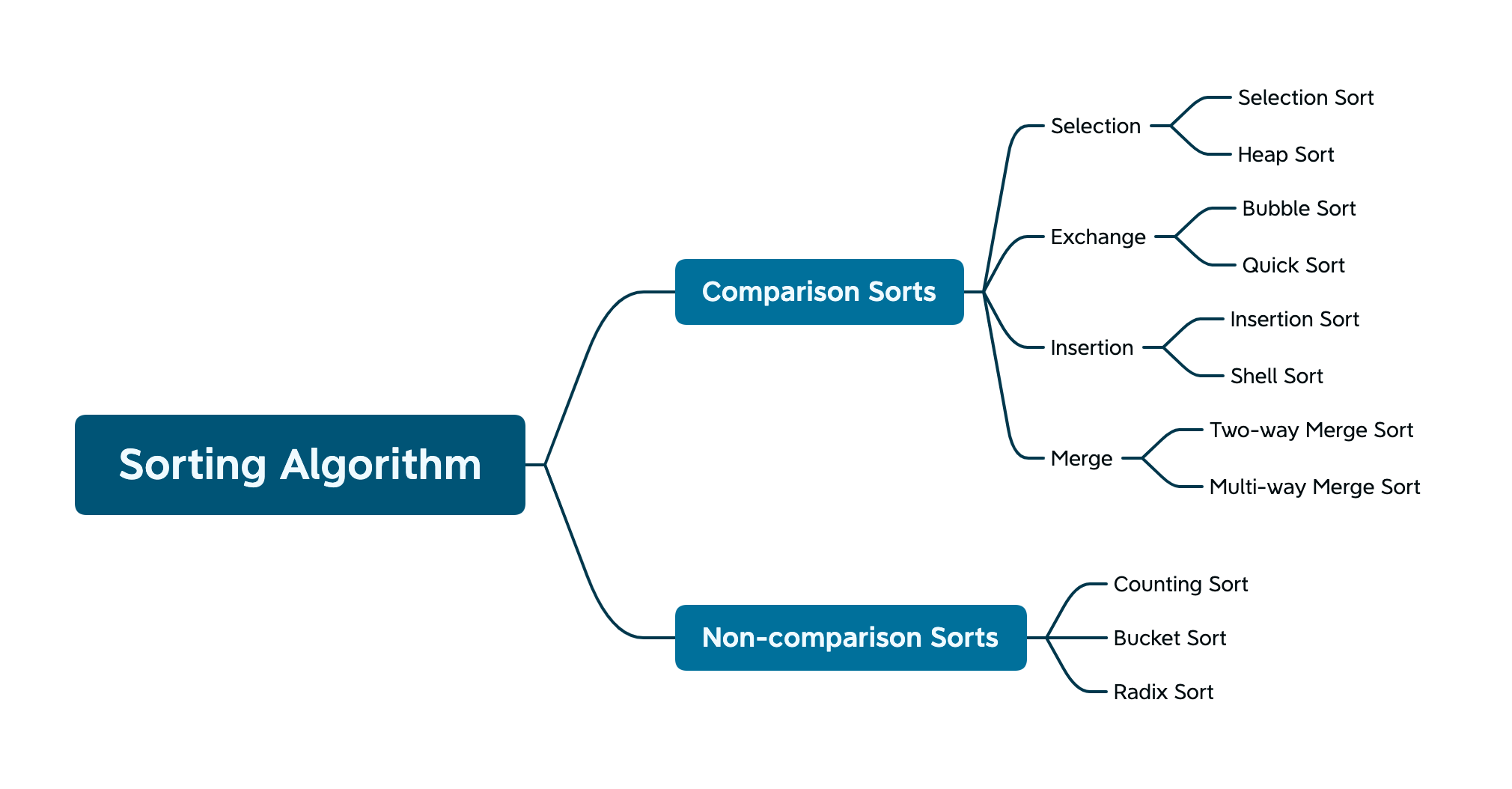
Sorting
Simple Sort:
- Selection
- Insertion
- Bubble
Efficient Sort:
- Heap
- Merge
- Quick
Sorting: Complexity
| sorting | avg | best | worst | inplacement | space | stability |
|---|---|---|---|---|---|---|
| Selection | O(n2) | O(n2) | O(n2) | in-place | O(1) | NOT stable |
| Insertion | O(n2) | O(n) 👍 | O(n2) | in-place | O(1) | stable |
| Bubble | O(n2) | O(n)* | O(n2) | in-place | O(1) | stable |
| Heap | O(nlogn) | O(nlogn) | O(nlogn) | in-place | O(1) | NOT stable |
| Merge | O(nlogn) | O(nlogn) → O(n)* | O(nlogn) | OUT-place | O(n) 👎 | stable |
| Quick | O(nlogn) | O(nlogn) → O(n)* | O(n2) 👈 | in-place | O(1) | NOT stable |
Sorting
| n2 | nlogn | faster | |
|---|---|---|---|
| n = 10 | 100 | 33 | 3 |
| n = 100 | 10,000 | 664 | 15 |
| n = 1,000 | 1,000,000 | 9,966 | 100 |
| n = 10,000 | 100,000,000 | 132,877 | 753 |
👉 1hr vs 31days (≈ 753hrs)
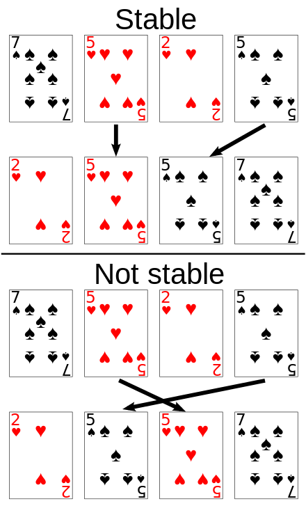
Sorting: stability
Stable sort algorithms sort equal elements in the same order that they appear in the input:
Sorting
Industrial Implementation
list.sort() or sorted(list)
| sorting | best | avg | worst |
|---|---|---|---|
| Merge | O(nlogn) | O(nlogn) | O(nlogn) |
| Quick | O(nlogn) | O(nlogn) | O(n2) |
| Timsort | O(n) 👈 | O(nlogn) | O(nlogn) |
✅ size < 64 → insertion sort
✅ otherwise → "adaptive merge sort"
2 types of sorting operations:
- moving or coping objects (just one step)
- comparing two objects:compare class type → compare method → if not, …
⚠️ comparing objects is very expensive
Industrial Implementation
list.sort() or sorted(list)
- run: parts that are strictly increasing (if decreasing, reverse it)
- split into multiple runs
- Galloping: merge runs
[1, 2, 3, ..., 100, ..., 101, 102, 103, ..., 200]
run1 = [1, 2, 3, , ..., 100]
run2 = [101, 102, 103, , ..., 200]
......
run2[2n−1−1]≤run1[0]≤run2[2n−1]
binary search: O(N) → O(logN)
Industrial Implementation
Arrays.sort() or Collections.sort()
primitive array: Dual Pivot Quicksort
object array: Timsort
Selection
Selection
In computer science, a selection algorithm is an algorithm for finding the kth smallest number in a list or array; such a number is called the kth order statistic. This includes the cases of finding the minimum, maximum, and median elements.
🙂 sort the array first O(NlogN)
Select K
Heap
Solution 1: complexity O(N)+O(KlogN)
- heapify (Min Heap)
- pop k times (remove_min)
Solution 2: complexity O(K)+O(NlogK)
create a Max Heap with size k, add element one by one:
- if smaller than the top, replace it;
- else skip it
min()
Select K
Quick Sort
p = partition(arr, l, r)
sort_quick_recursive(arr, l, p - 1)
sort_quick_recursive(arr, p + 1, r)p = partition(arr, l, r)
sort_quick_recursive(arr, l, p - 1)
sort_quick_recursive(arr, p + 1, r)
k==p?
k<p?
k>p?
complexity O(n+n/2+n/4+...+1)=O(2n)=O(n)
Pruning
- brute force
- BFS
- DFS
- Do not visit any subtree that be judged to be irrelevant to the final results.
The elimination of a large group of possibilities in one step is known as pruning:
👉 binary search
👉 alpha-beta pruning
👉 decision tree pruning
Text Processing
Text Processing
Algorithms on Strings
docs editors, emails, messages
web sites, search engine
bio-data (genonme sequencing)
natual language processing (NLP)
…
Example:
“Hello World”
“http://www.google.com”
“CGTAAACTGCTTTAATCAAACGC”
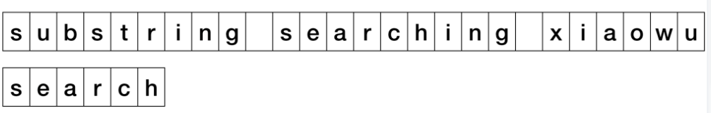
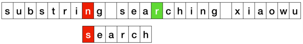
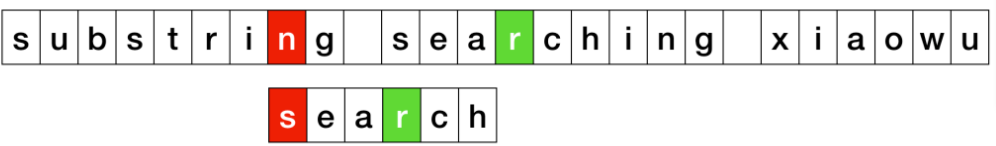
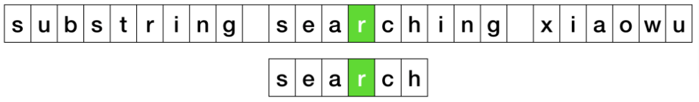
Pattern Matching
Pattern Matching
For a text string S with a length of n, and a pattern string P with length of m, decides if P is a substring of S.
Approximate Pattern Matching
input: a text string S with a length of n, a pattern string P with length of m, and an integer d
output: all positions in S where P appears as a substrign with at most d mismatches
Pattern Matching
Brute Force
Rabin-Karp (Michael O. Rabin and Richard M. Karp, 1987)
Knuth-Morris-Pratt Algorithm (KMP) (Knuth, Morris and Pratt, 1977)
Boyer-Moore Algorithm (BM) (Robert S. Boyer and J Strother Moore, 1970, 1974, 1977 )
Sunday Algorithm (Sunday) (Daniel M.Sunday, 1990)
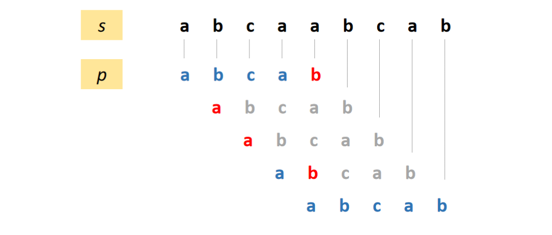
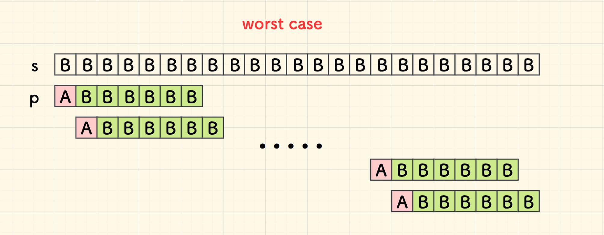
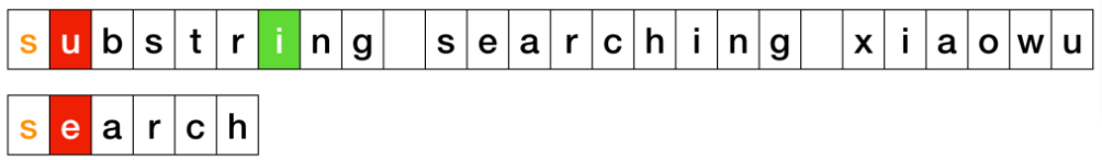
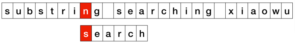
Brute Force
Brute Force
Rabin-Karp
Rabin-Karp
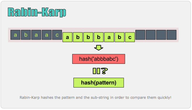
Rabin-Karp
Rolling Hash
S with a length of n, and a pattern string P with length of m
for i=m−1...n−1, compute hashing h(i) for substring S[i-m+1…i]:
B=256
M=1e9+7
BP=Bm−1%M
h(i-1): S[i-m+1] … S[i-1]
h(i): S[i-m+1] … S[i-1] S[i]
h[i]=(h∗B+S[i])%M
h=h[i−1]−s[i−m+1]∗Bm−1%M
h=(h[i−1]−s[i−m+1]∗Bm−1%M+M)%M ⏰
h=(h[i−1]−s[i−m+1]∗BP%M+M)%M
e.g. m = 5
"54321": 5∗104+4∗103+3∗102+2∗101+1∗100
"bbabc": b∗2564+b∗2563+a∗2562+b∗2561+c∗2560
(a+b)%M=(a%M+b%M)%M
(a∗b)%M=(a%M∗b%M)%M
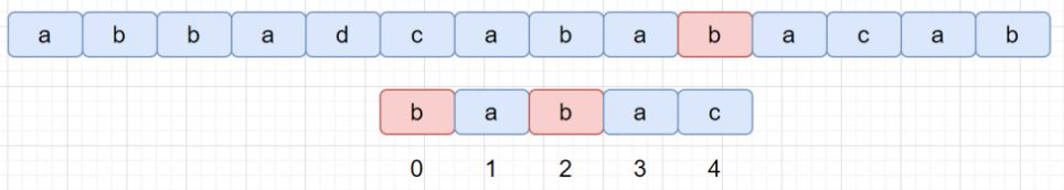
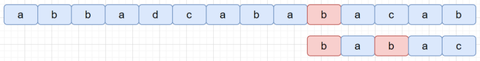
Knuth-Morris-Pratt
Knuth-Morris-Pratt (KMP)
prefix/suffix
| S | b | c | b | c | b | d | b | c | b | e |
| P | b | c | b | c | b | e | a |
| S | b | c | b | c | b | d | b | c | b | e | 👎 |
| P | b | c | b | c | b | e | a |
| S | b | c | b | c | b | d | b | c | b | e | 👍 |
| P | b | c | b | c | b | e | a |
longest common "prefix/suffix"
P: b c b c e a

prebuild the array to store the next position to shift for any substrings of P:
b, b c, b c b, b c b c, b c b c e, b c b c e
Knuth-Morris-Pratt (KMP)
next array
| substring | last pos | prefix last char | next pos |
|---|---|---|---|
| b | 0 | -1 | next[0] = -1 |
| b c | 1 | -1 | next[1] = -1 |
| b c b | 2 | 0 (b) | next[2] = 0 |
| b c b c | 3 | 1 (b c) | next[3] = 1 |
| b c b c b | 4 | 2 (b c b) | next[4] = 2 |
| b c b c b e | 5 | -1 | next[5] = -1 |
| S | b | c | b | c | b | d | b | c | b | e |
| P | b | c | b | c | b | e | a | |||
| j | 0 | 1 | 2 | 3 | 4 | 5 |
char to compare in pattern: j=5
bad char: P[5]
substring: P[0:5] (b c b c b)
look for longest common prefix/suffix: next[5−1]
next char to compare in pattern: j=next[5−1]+1=2+1=3
| S | b | c | b | c | b | d | b | c | b | e |
| P | b | c | b | c | b | e | a | |||
| j | 0 | 1 | 2 | 3 |
Knuth-Morris-Pratt (KMP)
for i = 0…n, compare S[i] and P[j]:
S[i]==P[j]
- if j=m, P is found in S
- else move both S and P to next char
i++, j++
S[i]!=P[j] (bad char)
- if longest common prefix/suffx found, next char to compare:
j=next[j−1]+1 - else compare from the begining (∵ next[j−1]=−1):
j=next[j−1]+1=−1+1=0
- if longest common prefix/suffx found, next char to compare:
for i in range(len_s):
        while j > 0 and s[i] != p[j]:
            # refer to slides: "bad char" found
            j = next_arr[j - 1] + 1
        if s[i] == p[j]:
            j += 1
        if j == len_p:
            return i - len_p + 1for i in range(len_s):
        while j > 0 and s[i] != p[j]:
            # refer to slides: "bad char" found
            j = next_arr[j - 1] + 1
        if s[i] == p[j]:
            j += 1
        if j == len_p:
            return i - len_p + 1
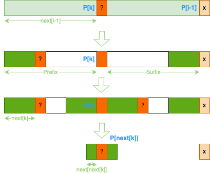
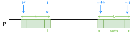
Knuth-Morris-Pratt (KMP)
next array
Give next[i−1]=k and P[i]=x then next[i]?
case1: P[k+1]==x, than next[i]=k+1
case2: if not, continuously look for k′, so that P[k′+1]==x
k: next[i−1] → next[k] → next[next[k]] → next[next[next[k]]] …
x?: P[k] → P[next[k]] → P[next[next[k]]] → …
while k != -1 and p[k + 1] != p[i]:
    k = next_arr[k]
if p[k + 1] == p[i]:
    k += 1
next_arr[i] = kwhile k != -1 and p[k + 1] != p[i]:
    k = next_arr[k]
if p[k + 1] == p[i]:
    k += 1
next_arr[i] = k
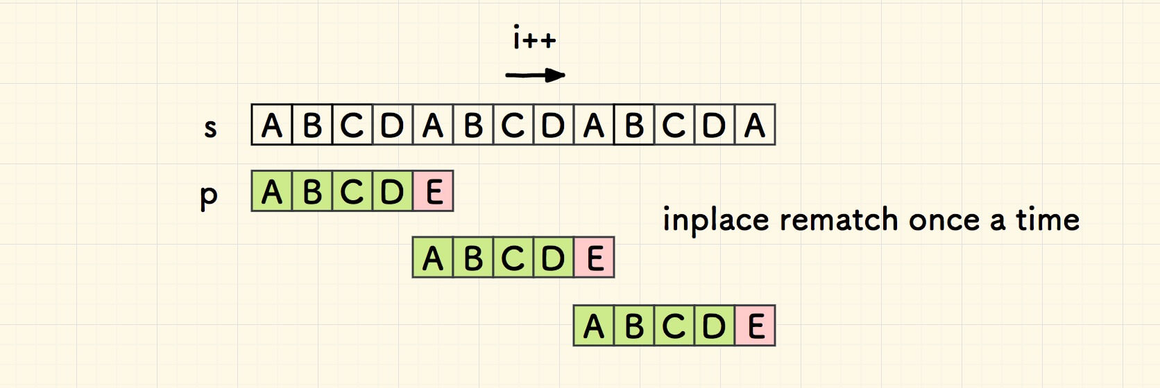
Knuth-Morris-Pratt (KMP)
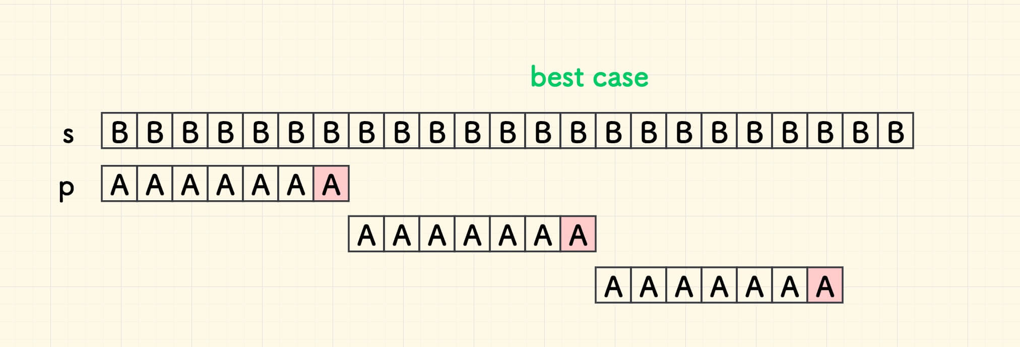
worst case: O(n+(m−1)∗n/m+m)
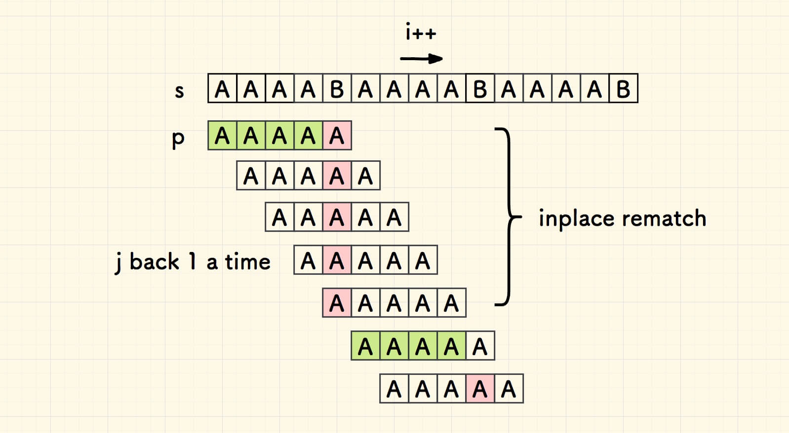
best case: O(n+1∗n/m+m)
Boyer-Moore
Boyer-Moore (BM)
bad char heuristic
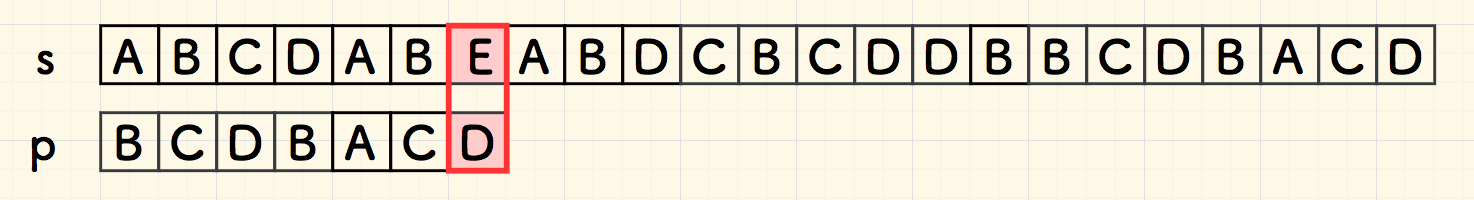
"bad char"
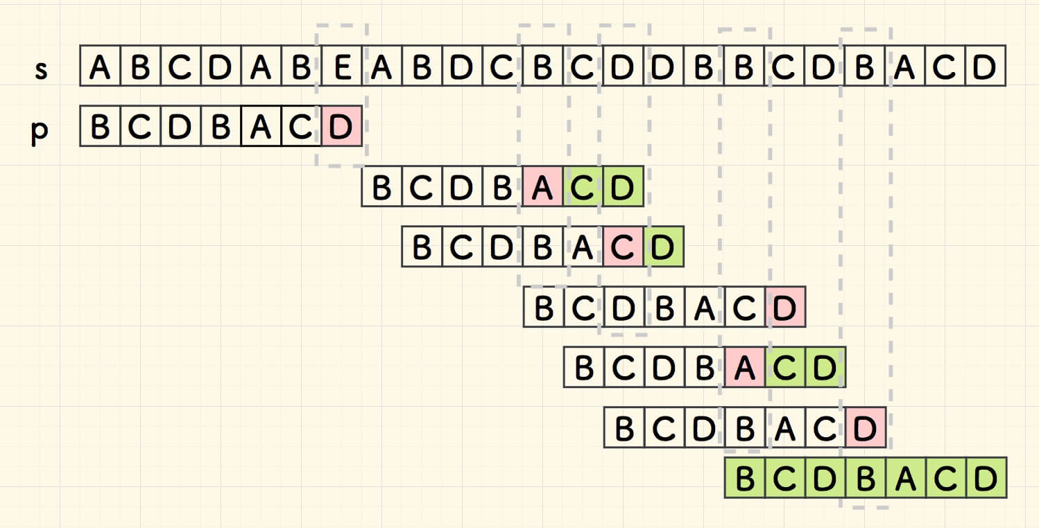
Boyer-Moore (BM)
bad char heuristic
look for the right most bad char:
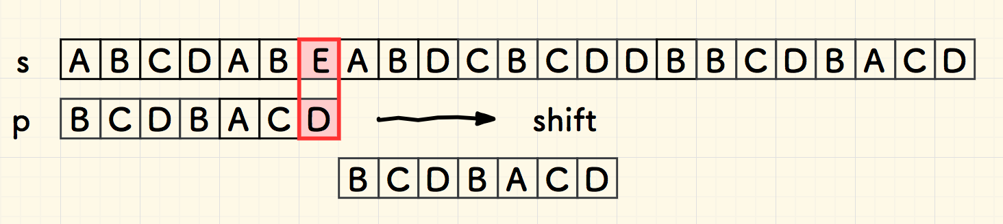
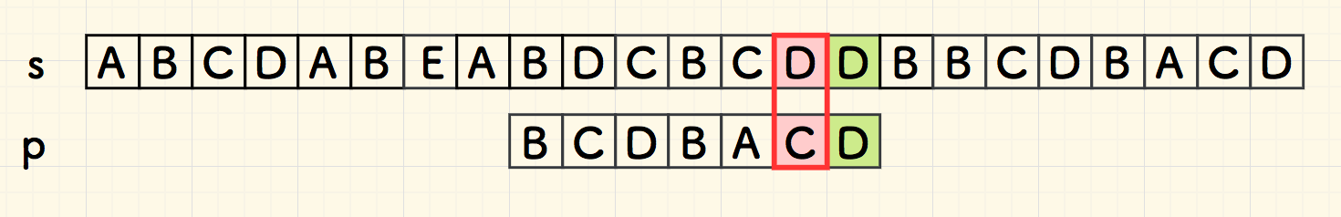
Boyer-Moore (BM)
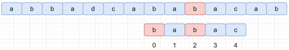
bad char heuristic
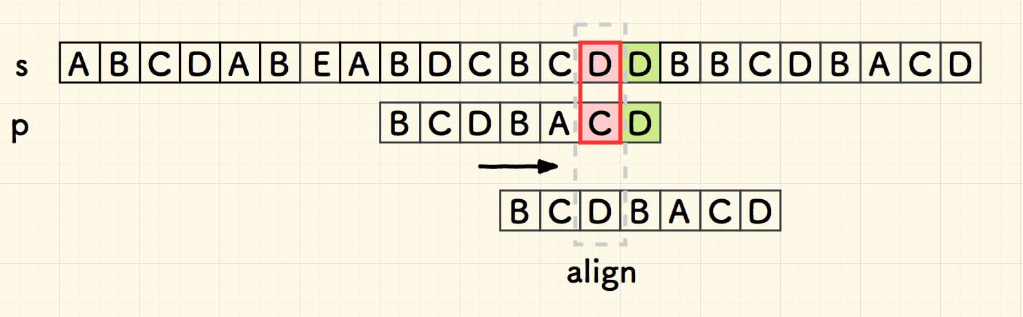
bad char shift d=j−b
- where S[i+j] is the bad char, and P[b]==S[i+j] is the right most bad char
- if P[b] doesnot exist, let b=−1
💬 bad char offset b can be pre-built for bad char position j (P[j]) for all possible missing char in 2-D lookup table badchar_tbl ?
| S | B | D | C | B | C | D | D | B | B | C | D |
| P | B | C | D | B | A | C | D | ||||
| j | 0 | 1 | 2 | 3 | 4 | 5 |
d=5−2=3
| S | B | D | C | B | C | D | D | B | B | C | D |
| i | 0 | 1 | 2 | 3 | |||||||
| P | B | C | D | B | A | C | D |
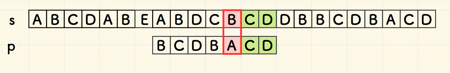
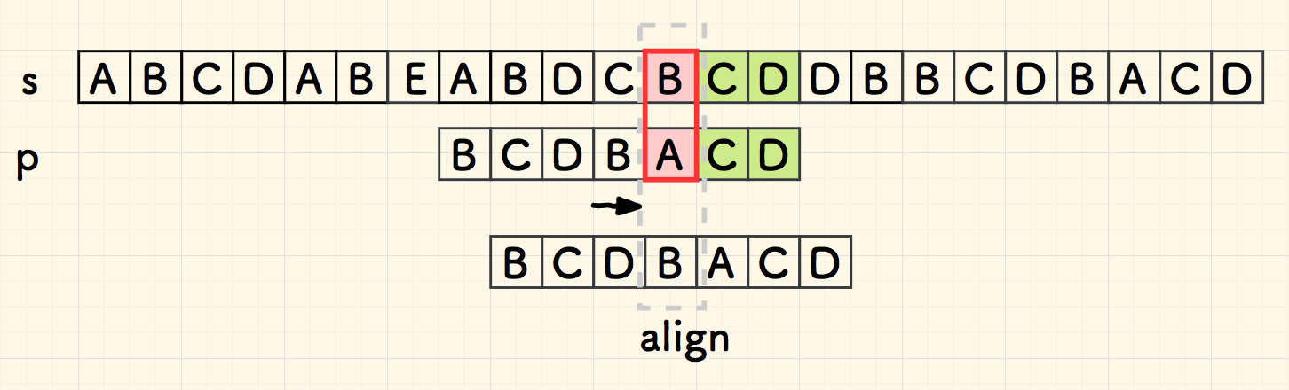
Boyer-Moore (BM)
bad char heuristic
let P[b] be the right most char regardless j
case1: bad char not found d=j−b=j−(−1)
case2: bad char found and b<j, d=j−b
case3: when d≤0, let d=1 (might not be the optimized shift)
| P | a | b | d | a |
| index | 0 | 1 | 2 | 3 |
badchar_tbl becomes 1-D table:
| bad char | 0 | 1 | ... | 97 | 98 | 99 | 100 | ... | 255 |
| b | -1 | -1 | ... | 3 | 1 | -1 | 2 | ... | -1 |
case1:
| S | a | b | c | d | e | f | g | f |
| P | e | f | g | f |
| S | a | b | c | d | e | f | g | f |
| P | e | f | g | f |
case2:
| S | a | b | a | e | c | d | g | f |
| P | a | e | c | d |
| S | a | b | a | e | c | d | g | f |
| P | a | e | c | d |
case3:
| S | a | a | a | a | a | a | a | a |
| P | b | a | a |
| S | a | a | a | a | a | a | a | a |
| P | b | a | a |
Boyer-Moore (BM)
good suffix heuristic
"good suffix"
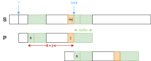
Boyer-Moore (BM)
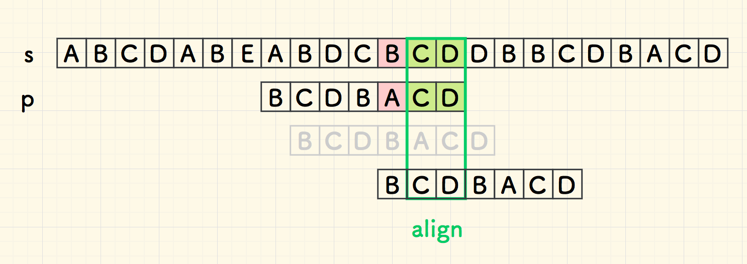
good suffix heuristic
good suffix on the left, shift d=j−s
- P[j]: bad char
- P[j+1:m] = P[s:s+k]: good suffix with length k=(m−1)−j
💬 good suffix with offset s for bad char P[j] can be pre-built in a suffix array
Boyer-Moore (BM)
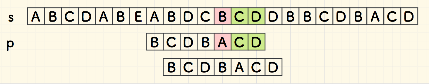
good suffix heuristic
good suffix NOT on the left, shift d=m ?
⚠️ Prefix
bad char: "c", good suffix: "d c a", prefix: "c a"
| S | a | b | c | b | d | c | a | d | c | d | c | a | c | c |
| P | c | a | d | c | d | c | a |
| S | a | b | c | b | d | c | a | d | c | d | c | a | c | c | ❌ |
| P | c | a | d | c | d | c | a |
| S | a | b | c | b | d | c | a | d | c | d | c | a | c | c | ✅ |
| P | c | a | d | c | d | c | a |
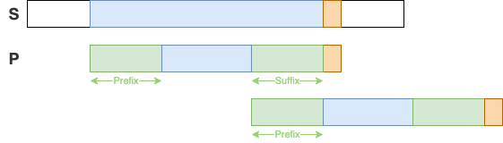
Boyer-Moore (BM)
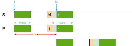
good suffix heuristic
a prefix in good suffix, shift d=r
- P[j]: bad char
- P[j+1:m]: good suffix
- P[j+2:m]: potential prefix
- P[r:m]: the largest prefix (P[0:m−r]), where j+2≤r≤m−1
💬 prefix for length m−r checking can be pre-built in a prefix array
Boyer-Moore (BM)
good suffix heuristic
- Suffix array: start position of the right most suffix
- Prefix array: True if it is a prefix
P: "abcdab"
| good suffix | len | suffix | prefix |
|---|---|---|---|
| b | 1 | suffix[1] = 1 | prefix[1] = false |
| ab | 2 | suffix[2] = 0 | prefix[2] = true |
| dab | 3 | suffix[3] = -1 | prefix[3] = false |
| cdab | 4 | suffix[4] = -1 | prefix[4] = false |
| bcdab | 5 | suffix[5] = -1 | prefix[5] = false |
def build_goodsuffix_arr(p):
    m = len(p)
    suffix = [-1 for _ in range(m)]
    prefix = [False for _ in range(m)]
    for i in range(m - 1):
        # two pointers to compare suffix
        j = i
        k = 0
        while j >= 0 and p[j] == p[m - 1 - k]:
            k += 1
            suffix[k] = j
            j -= 1
        if j == -1:
            prefix[k] = True
    return suffix, prefixdef build_goodsuffix_arr(p):
    m = len(p)
    suffix = [-1 for _ in range(m)]
    prefix = [False for _ in range(m)]
    for i in range(m - 1):
        # two pointers to compare suffix
        j = i
        k = 0
        while j >= 0 and p[j] == p[m - 1 - k]:
            k += 1
            suffix[k] = j
            j -= 1
        if j == -1:
            prefix[k] = True
    return suffix, prefix
Boyer-Moore (BM)
good suffix heuristic
- d=j−s (s: right most suffix offset)
- d=r (prefix P[r:m] true, where j+2≤r≤m−1)
- d=m (neither 1 or 2)
def search_bm_shift_goodsuffix(suffix, prefix, m, j):
    k =  m - 1 - j # length of good suffix
    # look for right most suffix with length k
    if suffix[k] != -1:
        # "suffix" exists
        return j - suffix[k] + 1
    # look for the largest prefix in P[j+2...m]: j+2 <= r <= m-1
    for r in range(j+2, m, 1):
        if prefix[m-r]:
            # "prefix" exists
            return r
    # no suffix, no prefix
    return mdef search_bm_shift_goodsuffix(suffix, prefix, m, j):
    k =  m - 1 - j # length of good suffix
    # look for right most suffix with length k
    if suffix[k] != -1:
        # "suffix" exists
        return j - suffix[k] + 1
    # look for the largest prefix in P[j+2...m]: j+2 <= r <= m-1
    for r in range(j+2, m, 1):
        if prefix[m-r]:
            # "prefix" exists
            return r
    # no suffix, no prefix
    return m
Boyer-Moore (BM)
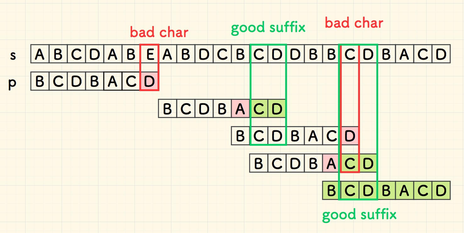
locate bad char P[j] then decide d:
bad char d1
good suffix d2
d=max(d1,d2)
# comapre backward to find "bad char"
for i in range(len_s - len_p + 1):
        j = len_p - 1
        # comapre backward to find "bad char"
        while j >= 0 and s[i+j] == p[j]:
            j -= 1
        if j < 0:
            # p is found
            return i
        # bad char found at s[i+j] != p[j]
        # bad char shift d1
        d1 = j - badchar_tbl[ord(s[i+j])]
        d1 = 1 if d1 <= 0 else d1
        # good suffix shift d2
        d2 = 0
        if len_p - 1 - j > 0:
            d2 = search_bm_shift_goodsuffix(suffix, prefix, len_p, j)
        i += max(d1, d2)# comapre backward to find "bad char"
for i in range(len_s - len_p + 1):
        j = len_p - 1
        # comapre backward to find "bad char"
        while j >= 0 and s[i+j] == p[j]:
            j -= 1
        if j < 0:
            # p is found
            return i
        # bad char found at s[i+j] != p[j]
        # bad char shift d1
        d1 = j - badchar_tbl[ord(s[i+j])]
        d1 = 1 if d1 <= 0 else d1
        # good suffix shift d2
        d2 = 0
        if len_p - 1 - j > 0:
            d2 = search_bm_shift_goodsuffix(suffix, prefix, len_p, j)
        i += max(d1, d2)
Boyer-Moore (BM)
Time Complexity
- best case: O(m+n/m)
- worst case: O(m+n∗m) 👉 ≈3n, see linkes below
Space Complexity:
- bad char table: O(256∗m) or O(m)
- suffix: O(m)
- prefix: O(m)
👉 A new proof of the linearity of the Boyer-Moore string searching algorithm
👉 Tight bounds on the complexity of the Boyer-Moore string matching algorithm
Sunday
Sunday
Complexity: KMP vs BM vs Sunday
| Pattern Matching | avg. | best | worst |
|---|---|---|---|
| KMP | O(m + n) | O(n) | O(m + n) |
| BP | O(m + n) | O(m + n/m) | O(m + n·m) |
| Sunday | O(m + n) | O(m + n/m) | O(m + n·m) |
👉 KMP always linear
Graph
Graph
- Implement graph ADT using different internal representation
- Learn graph associated algorithms
- How graph can be used to solve a wide variety of problems
💡 graph can model many things in real world such as roads, airline routes, social media connections, etc.
💡 graph theory, the study of graphs, is a field of discrete mathematics.
Graph Terminology
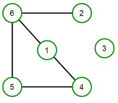
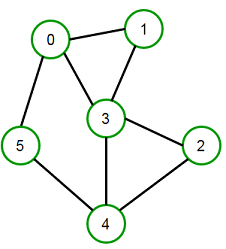
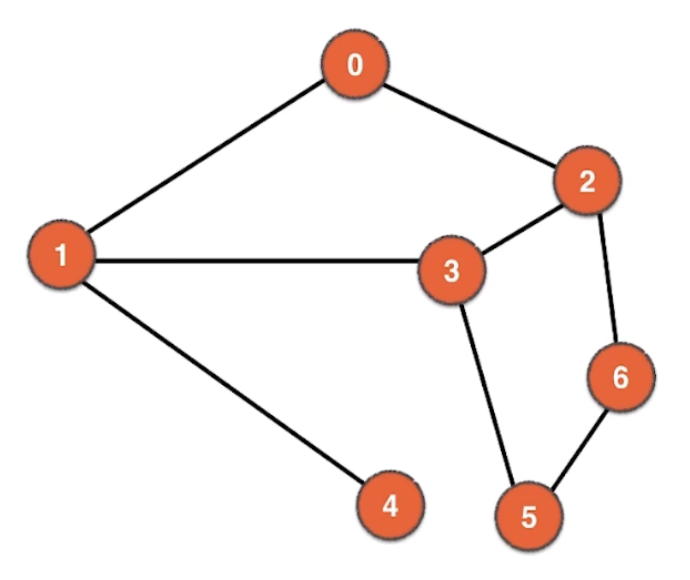
A graph is an ordered pair G=(V,E) comprising a set V of vertices or nodes and a collection of pairs of vertices from V, known as edges of a graph. For example, for the graph below:
V=1,2,3,4,5,6
E=(1,4),(1,6),(2,6),(4,5),(5,6)
Graph Terminology
- an edge is (together with vertices) one of the two basic units out of which graphs are constructed, each edge has two vertices to which it is attached, called its endpoints.
- two vertices are called adjacent or neighbors if they are endpoints of the same edge.
- outgoing edges of a vertex are directed edges that the vertex is the origin.
- incoming edges of a vertex are directed edges that the vertex is the destination.
- the degree of a vertex in a graph is the total number of edges incident to it.
- in a directed graph, the out-degree of a vertex is the total number of outgoing edges, and the in-degree is the total number of incoming edges.
- a vertex with in-degree zero is called a source vertex, while a vertex with out-degree zero is called a sink vertex.
- an isolated vertex is a vertex with degree zero, which is not an endpoint of an edge.
- if two or more undirected edges have the same two endpoint, or both origin and destination for two or more directed edges are the same, those edges are called parallel edges or multiple edges.
- if two endpoints for an edge are the same vertex, th edge become self-loop.
Graph Terminology
- path is a sequence of alternating vertices and edges such that the edge connects each successive vertex.
- if a path only has the directed edges and traverse along the edges’ direction, the path is called a directed path.
- path length is number of edges in a path.
- cycle is a path that starts and ends at the same vertex.
- simple path is a path with distinct vertices.
- two vertices are connected if a path exists between them.
- in a directed graph, if there is a path from vertex v to vertex w, it is said that w is reachable from v.
Graph Terminology
- a graph is connect when all vertices are connected.
- A connected component or simply component of an undirected graph is a subgraph in which each pair of nodes is connected with each other via a path.
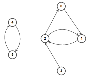
- a directed graph is strongly connected if for any pair of vertice v and w, w is reachable from v and v also reachable from w.
- a directed graph is called weakly connected if replacing all of its directed edges with undirected edges produces a connected (undirected) graph. The vertices in a weakly connected graph have either out-degree or in-degree of at least 1.
- if a graph H’s vertices and edges belong to a graph G’s vertices and edges, then graph H is a subgraph of G.
- if all vertices in G are in its subgraph H, then H is a spanning subgraph of G.
- a bridge is an edge whose removal would disconnect the graph.
- forest is a graph without cycles.
- tree is a connected graph with no cycles.
- if a spanning subgraph is a tree, then the spanning subgraph is called a spanning tree.
Graph Terminology
- root node is the ancestor of all other nodes in a graph. It does not have any ancestor. Each graph consists of exactly one root node. Generally, you must start traversing a graph from the root node.
- leaf node represents the node that do not have any successors. These nodes only have ancestor nodes. They can have any number of incoming edges but they will not have any outgoing edges.
Types of Graphs
Undirected and Directed Graph
An undirected graph(graph) is a graph in which edges have no orientation. The edge (x,y) is identical to edge (y,x), i.e., they are not ordered pairs. The maximum number of edges possible in an undirected graph without a loop is n×(n−1)/2.

social: friends
Types of Graphs
Undirected and Directed Graph
A directed graph (digraph) is a graph in which edges have orientations, i.e., The edge (x,y) is not identical to edge (y,x).
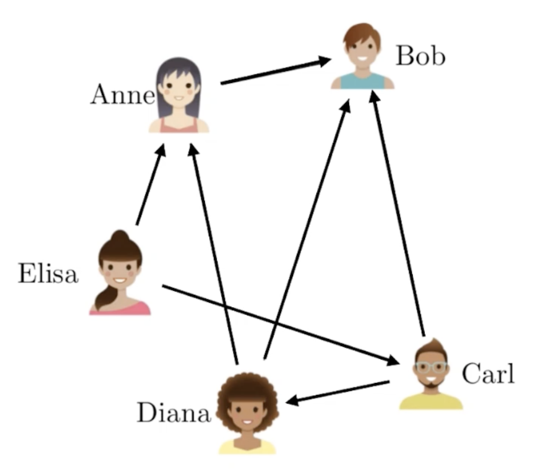
social: follows
Types of Graphs
Undirected and Directed Graph
A mixed graph has both undirected and directed edges.
Types of Graphs
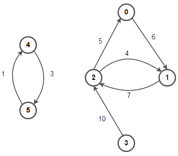
Weighted and Unweighted Graph
A weighted graph associates a value (weight) with every edge in the graph.
An unweighted graph does not have any value (weight) associated with every edge in the graph. In other words, an unweighted graph is a weighted graph with all edge weight as 1. Unless specified otherwise, all graphs are assumed to be unweighted by default.
Types of Graphs
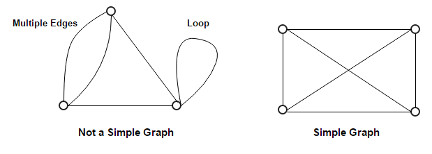
Simple and Multi Graph
A multigraph is an undirected graph in which multiple edges (and sometimes loops) are allowed.
A simple graph is an undirected graph in which both multiple edges and loops are disallowed as opposed to a multigraph. In a simple graph with n vertices, every vertex’s degree is at most n−1.
Types of Graphs
Connected Graph
A connected graph has a path between every pair of vertices. In other words, there are no unreachable vertices. A disconnected graph is a graph that is not connected.
Types of Graphs
Directed (Cyclic) Graph and DAG
A Directed Acyclic Graph (DAG) is a directed graph that contains no cycles.
Types of Graphs
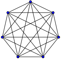
Complete Graph
A complete graph is one in which every two vertices are adjacent: all edges that could exist are present.
E=2V⋅(V−1)
Graph Properties
If a graph G has vertex set V and m edges, then vinV∑deg(v)=2m
If a directed graph G has vertex set V and m edges, then vinV∑indeg(v)=vinV∑outdeg(v)=m
A simple graph G has n vertices and m edges:
- undirected, then m≤n∗(n−1)/2
- directed, then m≤n∗(n−1)
An undirected graph G has n vertices and m edges:
- connected, then m≥(n−1)
- tree, then m=(n−1)
- forest, then m≤(n−1)
Graph ADT
Adjacency Matrix Representation
An adjacency matrix is a square matrix used to represent a finite graph. The elements of the matrix indicate whether pairs of vertices are adjacent or not in the graph. For a simple unweighted graph with vertex set V, the adjacency matrix is a square ∣V∣×∣V∣ matrix A such that its element:
Aij=1, when there is an edge from vertex Vi to vertex Vj, and
Aij=0, when there is no edge.
Each row in the matrix represents source vertices, and each column represents destination vertices. The diagonal elements of the matrix are all zero since edges from a vertex to itself, i.e., loops are not allowed in simple graphs. If the graph is undirected, the adjacency matrix will be symmetric. Also, for a weighted graph, Aij can represent edge weights.

Graph ADT
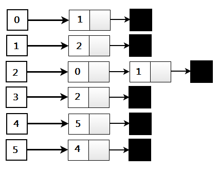
Adjacency List Representation
An adjacency list representation for the graph associates each vertex in the graph with the collection of its neighboring vertices or edges, i.e., every vertex stores a list of adjacent vertices. There are many variations of adjacency list representation depending upon the implementation. This data structure allows the storage of additional data on the vertices but is practically very efficient when the graph contains only a few edges. i.e. the graph is sparse.
Graph ADT
vertex_count()
edge_count()
vertices()
edges()
get_edge(vi, vj)
degree(v, out=True), degree(v, out=False)
incident_edge(v, out=True), incident_edge(v, out=False)
insert_vertex(w=None)
insert_edge(vi,vj,e=None)
remove_vertex(v)
remove_edge(e)
Graph ADT
| Space Complexity | construction | has_edge | adj | |
|---|---|---|---|---|
| Adjacency Matrix | O(V^2) | O(E) | O(1) | O(V) 👈 |
| Adjacency List | O(V + E) | O(E), O(E * V) | O(deg(v)), O(V) | O(deg(v)), O(V) |
Red-Black Tree?
HashSet?
Depth-First Search (DFS)
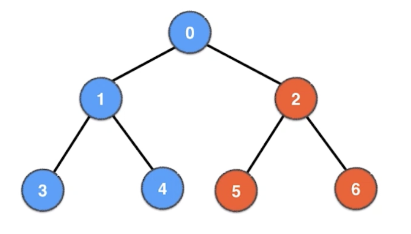
Depth-First Search (DFS)
preorder(root)

preorder(TreeNode node):
  if node != None:
    list.add(node.val)
    preorder(node.left)
    preorder(node.right)preorder(root)

preorder(TreeNode node):
  if node != None:
    list.add(node.val)
    preorder(node.left)
    preorder(node.right)
visited[0..V-1] = false
dfs(0)

dfs(int v):
  visited[v] = true
  list.add(v)
  for (int w: incident_edges(v)):
    if !visited[w]:
      dfs(w)visited[0..V-1] = false
dfs(0)

dfs(int v):
  visited[v] = true
  list.add(v)
  for (int w: incident_edges(v)):
    if !visited[w]:
      dfs(w)
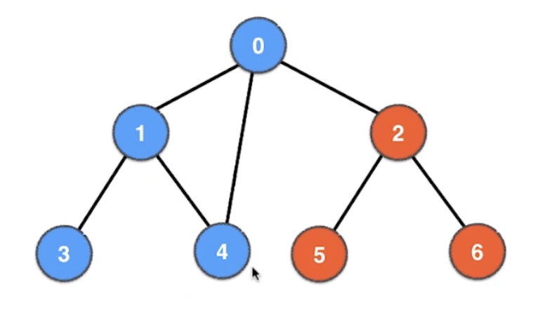
Depth-First Search (DFS)
visited[0..V-1] = false
dfs(0)

dfs(int v):
  visited[v] = true
  list.add(v)
  for (int w: incident_edges(v)):
    if !visited[w]:
      dfs(w)visited[0..V-1] = false
dfs(0)

dfs(int v):
  visited[v] = true
  list.add(v)
  for (int w: incident_edges(v)):
    if !visited[w]:
      dfs(w)
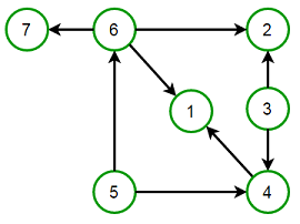
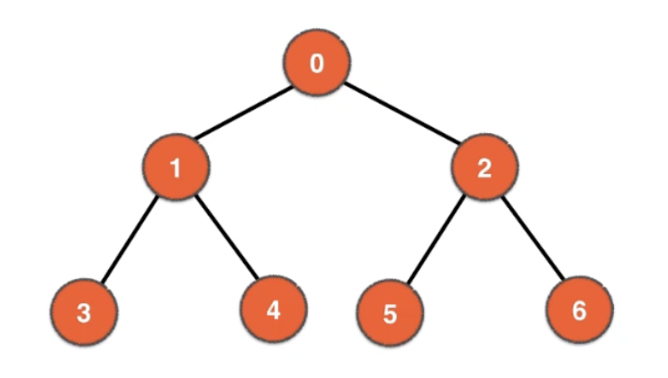
dfs(0) → dfs(1) → dfs(3) → dfs(2) → dfs(6) → dfs(5)
dfs(0) → dfs(1)
dfs(0) → dfs(1) → dfs(4)
list: 0 1 3 2 6 5 4
O(V+E)
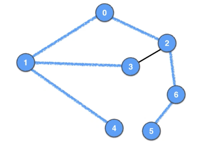
0 : 1 2
1 : 0 3 4
2 : 0 3 6
3 : 1 2 5
4 : 1
5 : 3 6
6 : 2 5
Depth-First Search (DFS)
prev[]:
1 ← 0
2 ← 3
3 ← 1
4 ← 1
6 ← 2
path from 0 to 6: 6 ← 2 ← 3 ← 1 ← 0
Depth-First Search (DFS)
- connected component
- a path between two vertices → Shortest path, Eulerian graph, Eulerian cycle, Hamiltonian path
- check cycle
- check a bipartite graph
- find bridge
- Tarjan’s strongly connected components algorithm
- …
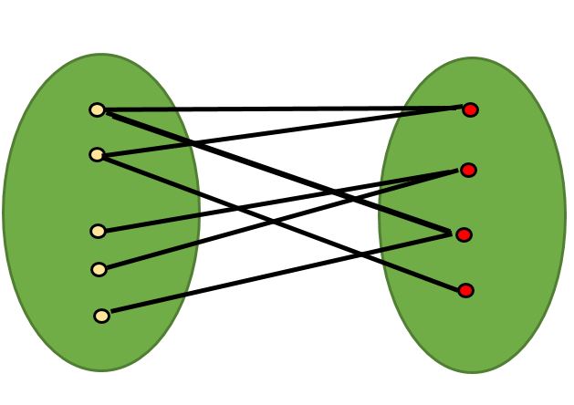
a bipartite graph (or bigraph) is a graph whose vertices can be divided into two disjoint and independent sets U and V, that is every edge connects a vertex in U to one in V.
Breadth-First Search (BFS)
Queue
0 :
2 → 1 : 0
4 → 3 → 2 : 1
6 → 5 → 4 → 3 : 2
6 → 5 → 4 : 3
6 → 5 : 4
6 : 5
: 6
BFS order: 0 1 2 3 4 5 6
Breadth-First Search (BFS)
Queue
0 :
2 → 1 : 0
4 → 3 → 2 : 1
6 → 4 → 3 : 2
5 → 6 → 4 : 3
5 → 6 : 4
5 : 6
: 5
BFS order: 0 1 2 3 4 6 5
O(V+E)
Depth-First Search (DFS)
👉 shortest path
Dijkstra’s Algorithm
Each iteration:
- from unvisited vertices, find the best vertex with shortest distance
- mark this vertex visited
- from this vertex, update distance to other unvisited vertices
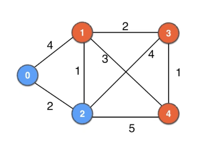
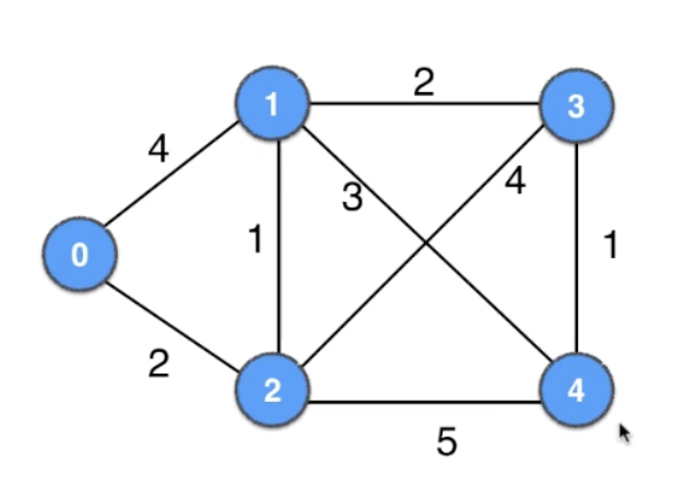
| 0 | 1 | 2 | 3 | 4 |
| 0 | ∞ | ∞ | ∞ | ∞ |
| 0 | 4 | 2 | ∞ | ∞ |
| 0 | 3 | 2 | 6 | 7 |
| 0 | 3 | 2 | 6 | 7 |
| 0 | 3 | 2 | 5 | 6 |
| 0 | 3 | 2 | 5 | 6 |
| 0 | 3 | 2 | 5 | 6 |
Path (0 —> 1): Minimum cost = 3, Route = [0, 2, 1]
Path (0 —> 2): Minimum cost = 2, Route = [0, 2]
Path (0 —> 3): Minimum cost = 5, Route = [0, 2, 1, 3]
Path (0 —> 4): Minimum cost = 6, Route = [0, 2, 1, 4]
Depth-First Search (DFS)
Space Complexity: O(V)
Time Complexity: O(V2) → O(ElogV) → O(E+VlogV)
shortest path from src to dest
all possible shortest path: O(V∗ElogV)
negative weight?
👉 Bellman-Ford
👉 Floyd–Warshall
Min-Spanning Tree (MST)
Spanning Tree: DFS & BFS
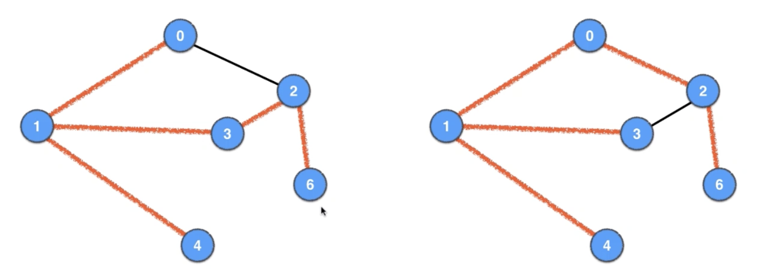
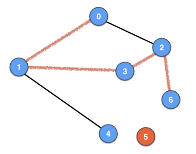
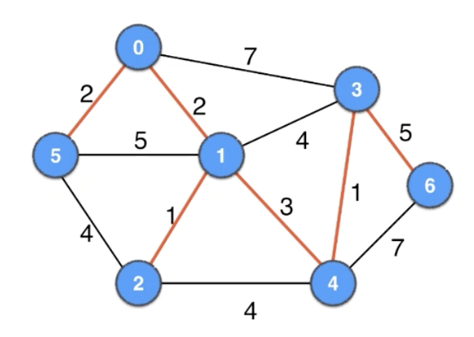
Kruskal’s Algorithm
repeatedly add the next lightest edge if this doesn’t producea cycle
greedy algorithm
1, 2: 1
3, 4: 1
0, 1: 2
0, 5: 2
1, 4: 3
1, 3 ❌   2, 4 ❌   2, 5 ❌
3, 6: 5
0, 3 ❌   4, 6 ❌
The Cut Property
In graph theory, a cut can be defined as a partition that divides a graph into two disjoint subsets.
A cut C=(S1,S2) in a connected graph G(V,E), partitions the vertex set V into two disjoint subsets S1, and S2.
A cut set of a cut C(S1,S2) of a connected graph G(V,E) can be defined as the set of edges that have one endpoint in S1 and the other in S2. For example the C(S1,S2) of G(V,E)=(i,j)∈E∣i∈S1,j∈S2
An edge is a crossing edge as an edge which connects a node from one set to a node from the other set.
👉 bipartitie graph: find a cut, so that every edge is crossing edge
The Cut Property
According to the cut property, given any cut, the minimum weight crossing edge is in the MST.
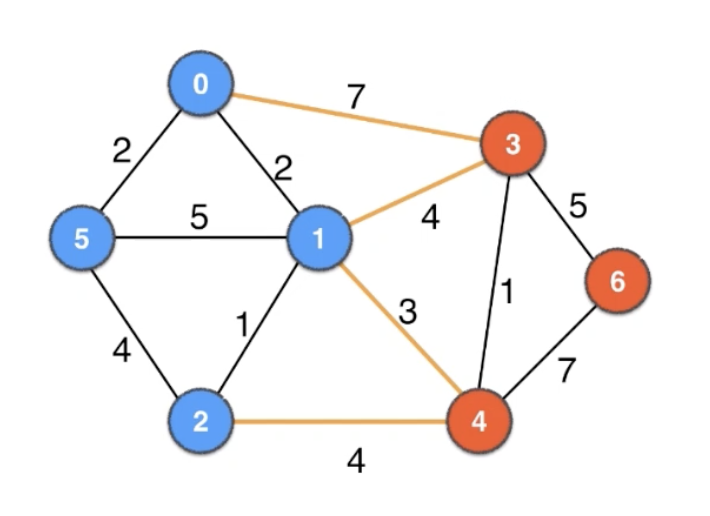
    0, 3: 7
    1, 3: 4
    1, 4: 3 👈
    2, 4: 4
Kruskal’s Algorithm
🙇🏻♂️ implementation
O(ElogE)
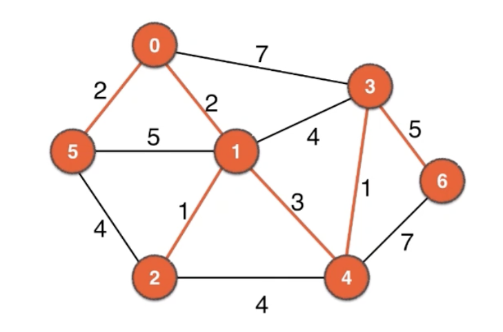
Prim’s Algorithm
start from 0, find the lightest crossing edge, and repeatly expand the cut
greedy algorithm
0, 1: 2   S1 = 0
1, 2: 1   S1 = 0, 1
0, 5: 2   S1 = 0, 1, 2
1, 4: 3   S1 = 0, 1, 2, 5
3, 4: 1   S1 = 0, 1, 2, 5, 4
3, 6: 5   S1 = 0, 1, 2, 5, 4, 3
             S1 = 0, 1, 2, 5, 4, 3, 6
Prim’s Algorithm
🙇🏻♂️ implementation
O(V2), O(ElogV), O(ElogE)
Min-Spanning Tree (MST)
Fedman-Tarjan O(E+VlogV)
- Fredman, M. L.; Willard, D. E. (1994), "Trans-dichotomous algorithms for minimum spanning trees and shortest paths", Journal of Computer and System Sciences, 48 (3): 533–551, doi:10.1016/S0022-0000(05)80064-9, MR 1279413.
Chazelle O(E∗)
- Chazelle, Bernard (2000), "A minimum spanning tree algorithm with inverse-Ackermann type complexity", Journal of the Association for Computing Machinery, 47 (6): 1028–1047, doi:10.1145/355541.355562, MR 1866456, S2CID 6276962.
- Chazelle, Bernard (2000), "The soft heap: an approximate priority queue with optimal error rate" (PDF), Journal of the Association for Computing Machinery, 47 (6): 1012–1027, doi:10.1145/355541.355554, MR 1866455, S2CID 12556140.
Algorithm Design Technique
Divide-and-Conquer
Input: Problem P
Algorithm divideAndConquer(P):
- Base case: if size of P is small, solve it (e.g. brute force) and return solution, else:
- Divide: divide P into smaller problems P1, P2
- Conquer: solve the smaller subproblems recursively, by calling divideAndConquer(P1) and divideAndConquer(P2)
- Combine: combine solutions to P1, P2 into solution for P.
Divide-and-Conquer
Merge-sort an array of n elements:
- base-case: if size of input is 1, return
- else:
- Divide: Divide the array into two arrays of n/2 elements each
- Conquer: Sort the two arrays recursively
- Combine: Merge the two sorted arrays of n/2 elements into one sorted array of size n
Greedy Algorithm
A greedy algorithm is a simple and efficient algorithmic approach for solving any given problem by selecting the best available option at that moment of time, without bothering about the future results.
To create greedy algorithm:
- Firstly, the solution set (that is supposed to contain answers) is set to empty.
- Secondly, at each step, an item is pushed to the solution set.
- Only if the solution set is deemed feasible, the current item is kept for future purpose.
- Else, the current item is rejected and is never considered again (no reversal of decision)
Greedy Algorithm
0-1 Knapsack: greedy and most valuable item?
w=[1,2,3], v=[6,10,12], C=5
| 0 | 1 | 2 | |
|---|---|---|---|
| weight | 1 | 2 | 3 |
| value | 6 | 10 | 12 |
| v/w | 6 | 5 | 4 |
6+10=16 ❌
10+12=22 ✅
Greedy Algorithm
Given an array of intervals intervals where intervals[i] = [starti, endi], return the minimum number of intervals you need to remove to make the rest of the intervals non-overlapping.
Input: intervals = [[1,2],[2,3],[3,4],[1,3]]
Output: 1
Explanation: [1,3] can be removed and the rest of the intervals are non-overlapping.
Input: intervals = [[1,2],[1,2],[1,2]]
Output: 2
Explanation: You need to remove two [1,2] to make the rest of the intervals non-overlapping.
Greedy: sort endi, select the smaller endi and non-overlapping intervals[i]
why correct?
Backtracking
- Backtracking Backtracking is an algorithmic technique for finding all solutions to some computational problems that have certain constraints and incrementally builds candidates to the solutions while abandoning a candidate if it does not lead to valid solutions.
- It is known for solving problems recursively one step at a time and removing those solutions that that do not satisfy the problem constraints at any point of time.
- It is a refined brute force approach that tries out all the possible solutions and chooses the best possible ones out of them.
- The backtracking approach is generally used in the cases where there are possibilities of multiple solutions.
Backtracking: Sudoku
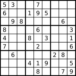
Input
[["5","3",".",".","7",".",".",".","."],
["6",".",".","1","9","5",".",".","."],
[".","9","8",".",".",".",".","6","."],
["8",".",".",".","6",".",".",".","3"],
["4",".",".","8",".","3",".",".","1"],
["7",".",".",".","2",".",".",".","6"],
[".","6",".",".",".",".","2","8","."],
[".",".",".","4","1","9",".",".","5"],
[".",".",".",".","8",".",".","7","9"]]
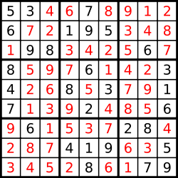
Output
[["5","3","4","6","7","8","9","1","2"],
["6","7","2","1","9","5","3","4","8"],
["1","9","8","3","4","2","5","6","7"],
["8","5","9","7","6","1","4","2","3"],
["4","2","6","8","5","3","7","9","1"],
["7","1","3","9","2","4","8","5","6"],
["9","6","1","5","3","7","2","8","4"],
["2","8","7","4","1","9","6","3","5"],
["3","4","5","2","8","6","1","7","9"]]
Backtracking
backtracking vs brute force:
- brute force algorithms are those which computes every possible solution to a problem and then selects the best one among them that fulfills the given requirements.
- Whereas, backtracking is a refined brute force technique where the implicit constraints are evaluated after every choice (not as in brute force where evaluation is done after all solutions have been generated). This means that potential non-satisfying solutions can be rejected before the computations have been ‘completed’.
backtracking vs recursion:
- In recursion, a function simply calls itself until reaches a base case.
- Whereas, in backtracking we use recursion for exploring all the possibilities until we get the best and feasible result for any given problem.
Dynamic Programming
Dynamic Programming (DP) is a method for solving a complex problem by breaking it down into a collection of simpler subproblems, solving each of those subproblems just one, and storing their solutions - ideally, using a memory-based data structure.
Writes down "1+1+1+1+1+ =" on a sheet of paper.
"What’s that equal to?"
Counting "Five!"
Writes down another "1+" on the left.
"What about that?"
"Six!" " How’d you know it was nine so fast?"
"You just added one more!"
"So you didn’t need to recount because you remembered there were five!
Dynamic Programming is just a fancy way to say remembering stuff to save time later!"
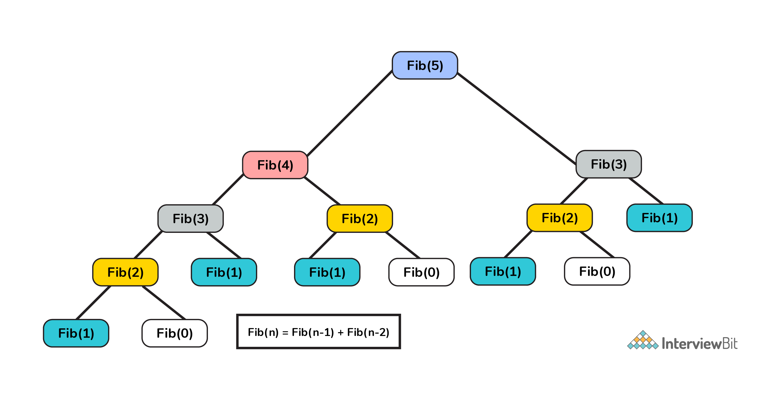
DP: Fibonacci
Fibonacci sequence: 0,1,1,2,3,5,8, ...

when n = 1, fib(1) = 0
when n = 2, fib(2) = 1
when n > 2, fib(n) = fib(n-1) + fib(n-2)Fibonacci sequence: 0,1,1,2,3,5,8, ...

when n = 1, fib(1) = 0
when n = 2, fib(2) = 1
when n > 2, fib(n) = fib(n-1) + fib(n-2)
# Time Complexity: O(2^n)
def fib_recursive(n):
    global fib_run
    fib_run += 1
    if (n == 1):
        return 0
    if (n == 2):
        return 1
    return fib_recursive(n-1) + fib_recursive(n-2)# Time Complexity: O(2^n)
def fib_recursive(n):
    global fib_run
    fib_run += 1
    if (n == 1):
        return 0
    if (n == 2):
        return 1
    return fib_recursive(n-1) + fib_recursive(n-2)
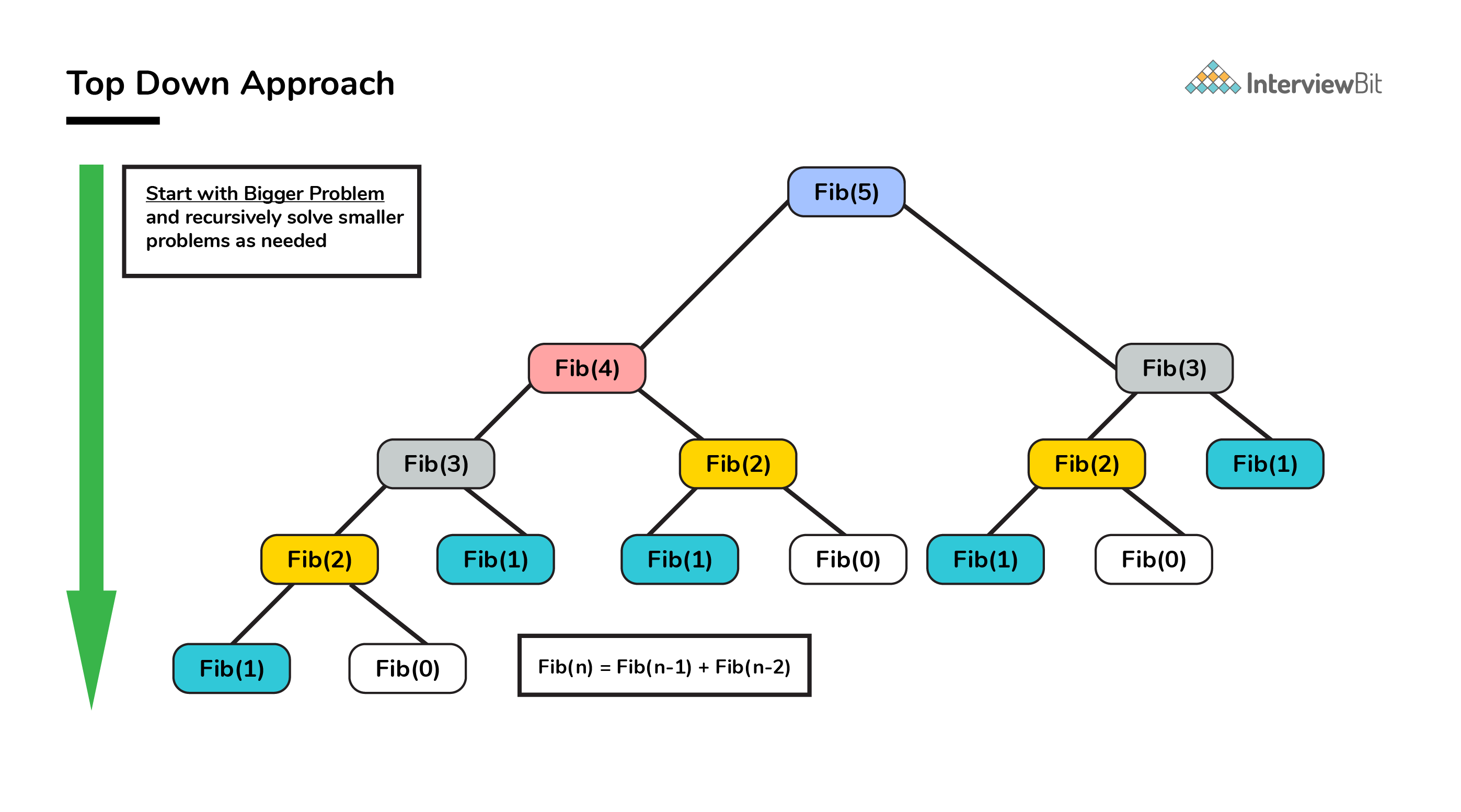
DP: Fibonacci
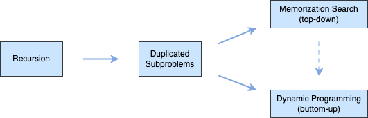
Any problem is said to have overlapping subproblems if calculating its solution involves solving the same subproblem multiple times.
This method of remembering the solutions of already solved subproblems is called Memoization.
# Time Complexity: O(n)
def fib_recursive_memo(n):
    global fib_run, fib_memo
    fib_run += 1
    # return directly from cache if found
    if (n in fib_memo):
        return fib_memo[n]
    if (n == 1):
        return 0
    if (n == 2):
        return 1
    # cache the result
    fib_memo[n] = fib_recursive_memo(n-1) + fib_recursive_memo(n-2)
    return fib_memo[n]# Time Complexity: O(n)
def fib_recursive_memo(n):
    global fib_run, fib_memo
    fib_run += 1
    # return directly from cache if found
    if (n in fib_memo):
        return fib_memo[n]
    if (n == 1):
        return 0
    if (n == 2):
        return 1
    # cache the result
    fib_memo[n] = fib_recursive_memo(n-1) + fib_recursive_memo(n-2)
    return fib_memo[n]
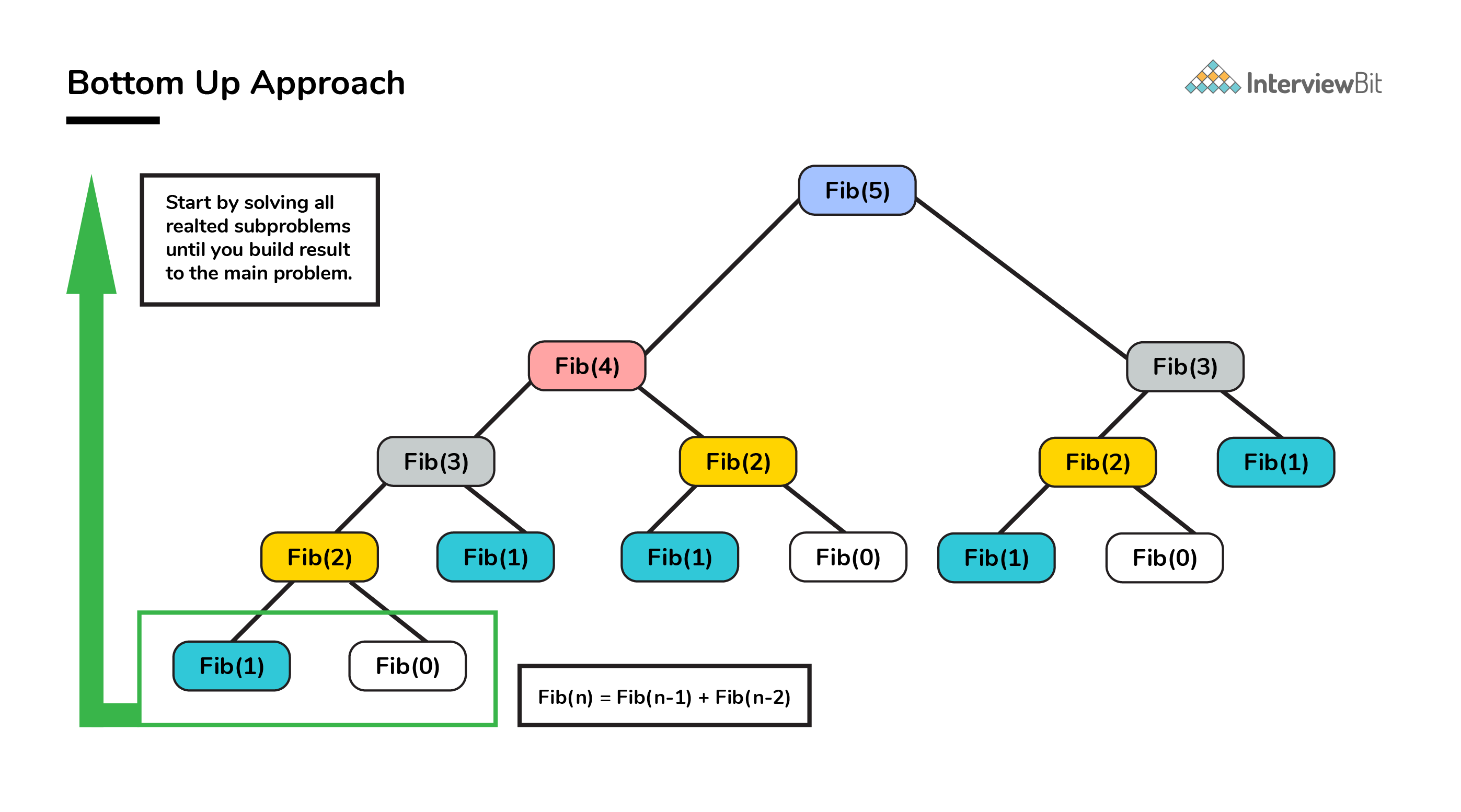
DP: Fibonacci
bottom up is the opposite of the top-down approach which avoids recursion by solving all the related subproblems first.
# Time Complexity: O(n)
def fib_dp(n):
    dp_memo = {}
    dp_memo[0] = 0
    dp_memo[1] = 0
    dp_memo[2] = 1
    for i in range(2, n+1, 1):
        dp_memo[i] = dp_memo[i-1] + dp_memo[i-2]
    return dp_memo[n]# Time Complexity: O(n)
def fib_dp(n):
    dp_memo = {}
    dp_memo[0] = 0
    dp_memo[1] = 0
    dp_memo[2] = 1
    for i in range(2, n+1, 1):
        dp_memo[i] = dp_memo[i-1] + dp_memo[i-2]
    return dp_memo[n]
DP Solution
DP in a nutshell:
- check for optimal substructure and formulate the problem recursively, and
- use a table to “cache” the solutions to subproblems, in order to avoid recomputing them.
💡 usually DP problem is hard
💡 different DP through exercises
DP: 0-1 Knapsack Problem
Given weights and values of n items, put these items in a knapsack of capacity C to get the maximum total value in the knapsack. In other words, given two integer arrays v[0..n−1] and w[0..n−1] which represent values and weights associated with n items respectively. Also given an integer C which represents knapsack capacity, find out the maximum value subset of v such that sum of the weights of this subset is smaller than or equal to C. You cannot break an item, either pick the complete item or don’t pick it (0-1 property).
w=[10,20,30], v=[60,100,120], C=50
solution: 200
w=10; v=60;
w=20; v=100;
w=30; v=120;
w=(20+10); v=(100+60);
w=(30+10); v=(120+60);
w=(30+20); v=(120+100);
w=(30+20+10) > 50
DP: 0-1 Knapsack Problem
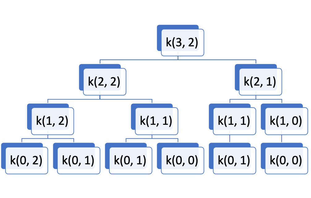
k(n,C): n items, capacity C, return max value
k(i,C):
- include ith item: v[i]+k(i−1,C−w[i])
- not included: k(i−1,C)
k(i,C)=max(k(i−1,C),v[i]+k(i−1,C−w[i]))
Time Complexity: O(2n)
w=[1,1,1]
v=[10,20,30]
C=2
DP: 0-1 Knapsack Problem
id=[0,1,2]
w=[1,2,3]
v=[6,10,12]
C=5
k(i,c)=max(k(i−1,c),v[i]+k(i−1,c−w[i]))
| 0 | 1 | 2 | 3 | 4 | 5 | |
|---|---|---|---|---|---|---|
| 0 | 0 | 6 | 6 | 6 | 6 | 6 |
| 1 | 0 | 6 | 10 | 16 | 16 | 16 |
| 2 | 0 | 6 | 10 | 16 | 18 | 22 |
Time Complexity: O(n)
Space Complexity: O(n∗C)
def knapsack2(w, v, n, C):
    k = [[0 for x in range(C+1)] for x in range(n+1)]
    # build table k from bottom up
    for i in range(n+1):
        for c in range(C+1):
            if i==0 or c==0:
                k[i][c] = 0
            elif w[i-1] > c:
                k[i][c] = k[i-1][c]
            else:
                k[i][c] = max(v[i-1] + k[i-1][c - w[i-1]], k[i-1][c])
    return k[n][C]def knapsack2(w, v, n, C):
    k = [[0 for x in range(C+1)] for x in range(n+1)]
    # build table k from bottom up
    for i in range(n+1):
        for c in range(C+1):
            if i==0 or c==0:
                k[i][c] = 0
            elif w[i-1] > c:
                k[i][c] = k[i-1][c]
            else:
                k[i][c] = max(v[i-1] + k[i-1][c - w[i-1]], k[i-1][c])
    return k[n][C]
DP: 0-1 Knapsack Problem
k(i,c)=max(k(i−1,c),v[i]+k(i−1,c−w[i]))
row i depends on row i−1, so only 2 rows required:
- row0 == even rows
- row1 == odd rows
Time Complexity: O(n)
Space Complexity: O(2∗C)
def knapsack3(w, v, n, C):
    # 2 rows only: i%2
    k = [[0 for x in range(C+1)] for x in range(2)]
    # build table k from bottom up
    for i in range(n+1):
        for c in range(C+1):
            if i==0 or c==0:
                k[i % 2][c] = 0
            elif w[i-1] > c:
                k[i % 2][c] = k[(i-1) % 2][c]
            else:
                k[i % 2][c] = max(v[i-1] + k[(i-1) % 2][c - w[i-1]], k[(i-1) % 2][c])
    return k[n % 2][C]def knapsack3(w, v, n, C):
    # 2 rows only: i%2
    k = [[0 for x in range(C+1)] for x in range(2)]
    # build table k from bottom up
    for i in range(n+1):
        for c in range(C+1):
            if i==0 or c==0:
                k[i % 2][c] = 0
            elif w[i-1] > c:
                k[i % 2][c] = k[(i-1) % 2][c]
            else:
                k[i % 2][c] = max(v[i-1] + k[(i-1) % 2][c - w[i-1]], k[(i-1) % 2][c])
    return k[n % 2][C]
DP: 0-1 Knapsack Problem
id=[0,1,2]
w=[1,2,3]
v=[6,10,12]
C=5
k(i,c)=max(k(i−1,c),v[i]+k(i−1,c−w[i]))
| 0 | 1 | 2 | 3 | 4 | 5 | |
|---|---|---|---|---|---|---|
| 0 | 6 | 6 | 6 | 6 | 6 |
| 0 | 1 | 2 | 3 | 4 | 5 | |
|---|---|---|---|---|---|---|
| 0 | 6 | 10 | 16 | 16 | 16 |
Time Complexity: O(n)
Space Complexity: O(C)
def knapsack4(w, v, n, C):
    k = [0 for i in range(C+1)]
    for i in range(1, n+1):
        # compute from the back (right to left)
        for c in range(C, 0, -1):
            if w[i-1] <= c:
                k[c] = max(v[i-1] + k[c - w[i-1]], k[c])
    return k[C]def knapsack4(w, v, n, C):
    k = [0 for i in range(C+1)]
    for i in range(1, n+1):
        # compute from the back (right to left)
        for c in range(C, 0, -1):
            if w[i-1] <= c:
                k[c] = max(v[i-1] + k[c - w[i-1]], k[c])
    return k[C]
DP: Egg Drop
You are given k identical eggs and you have access to a building with n floors labeled from 1 to n.
You know that there exists a floor f where 0<=f<=n such that any egg dropped at a floor higher than f will break, and any egg dropped at or below floor f will not break.
In each move, you may take an unbroken egg and drop it from any floor x (where 1<=x<=n). If the egg breaks, you can no longer use it. However, if the egg does not break, you may reuse it in future moves.
Return the minimum number of moves that you need to determine with certainty what the value of f is.
Input: k = 2, n = 100
Output: 14
DP: Egg Drop
- k=1: n
- k=∞: logN
- k=2 (A, B), n=100:
- A = 10, 20, 30, …, 100, B = x1, x2, x3, …, x9: 10 + 9 = 19 (not sure)
- A = 14, 27, 39, …, 95, 99, 100: 14 (not sure)
if drop at floor f:
- broken, floor[1...f−1]: drop(k−1,f−1)
- unbroken, floor[f+1...n]: drop(k,n−f)
we need to try: max(drop(k−1,f−1),drop(k,n−f))+1
so after try every floor f∈[1..n]
we can get the answer: min(max(dropf(k−1,f−1),dropf(k,n−f))+1))
drop m times: floor[k][m]=floor[k−1][m−1]+floor[k][m−1]+1
when floor[k][m]==n, m=?
DP vs Divide-and-Conquer
The most important difference in Divide and Conquer strategy is that the subproblems are independent of each other. When a problem is divided into subproblems, they do not overlap which is why each subproblem is to be solved only once.
Whereas in DP, a subproblem solved as part of a bigger problem may be required to be solved again as part of another subproblem (concept of overlapping subproblem), so the results of a subproblem is solved and stored so that the next time it is encountered, the result is simply fetched and returned.
DP vs Greedy
| Parameters | Dynamic Programming | Greedy Approach |
|---|---|---|
| Optimality | There is guaranteed optimal solution as DP considers all possible cases and then choose the best among them. | Provides no guarantee of getting optimum approach. |
| Memory | DP requires a table or cache for remembering and this increases it’s memory complexity. | More memory efficient as it never looks back or revises its previous choices. |
| Time complexity | DP is generally slower due to considering all possible cases and then choosing the best among them. | Generally faster. |
| Feasibility | Decision at each step is made after evaluating current problem and solution to previously solved subproblem to calculate optimal solution. | Choice is made which seems best at the moment in the hope of getting global optimal solution. |
Lab 1
Review "sift up" and "sift down" of MinHeap, implement your MaxHeap.
Give an O(logN * logN) algorithm to merge two binary heap.
Design a Min-Max Heap that supports both remove_min and remove_max in O(logN) per operation.
- how to find min and max element?
- how to insert/add an element?
- how to build a Min-Max Heap(heapify) in linear time?
Implement a classic Cuckoo Hash Table (Cuckoo hashing) and support the basic operations: insert, get and remove a key.
Lab 2
Implement BST search operation with iterative solution.
before(k) & after(k) in BST would not work if BST doesnot contain the key k, pls improve the algorithm to support such case.
(a) convert a BST into a MinHeap
(b) convert a MinHeap into a BSTOptimize AVL tree so when there is no change to the hight of nodes, the rebalance process can be stopped.
Implement a map data structure with AVL tree and support the basic operations: insert, get and remove a key.
Lab 3
Implement your Insertion Sort and sort the number array from right to left.
Implement your Bubble Sort and sort the number array from left to right.
Implement your Merge Sort and use bottom-up approach.
Shell Sort is an optimization of Insertion Sort. Implement your Shell Short.
Dual Pivot Quick Sort by Vladimir Yaroslavskiy, Jon Bentley, and Joshua Bloch, this algorithm offers O(NlogN) performance on many data sets that cause other quicksorts to degrade to quadratic performance, and is typically faster than traditional (one-pivot) Quicksort implementations. Implement your Dual Pivot Quick Sort.
Lab 4
Review KMP and implementate your solution
Review BM and implementate your solution
Lab 5
Iterative implementation of DFS with Adjacency List
Iterative implementation of BFS with Adjacency List
Modify DFS to detect cycle in undirected graph
Modify BFS to find a path (Single Source Shortest Path) in a undirected graph
Implement your Dijkstra algorithm with WeightdeGraph class
Implement your Kruskal algorithm with WeightdeGraph class
Implement your Prim algorithm with WeightdeGraph class
Lab 6
Q&A